Abstract
Background:
Accurate differentiation of angiomyolipoma (AML) from renal cell carcinoma (RCC) is important in RCC diagnosis.Objectives:
This study aimed to evaluate the performance of different supervised machine learning (ML) algorithms for RCC based on computed tomography (CT) examinations.Patients and Methods:
The CT images of known cases of RCC or renal AML were collected and divided into training and testing groups. The texture features of CT images were drawn and quantified in MaZda software; a total of 352 features were drawn from each image. Top 10 features with statistical significance for differentiation of RCC from benign tumors in the training group were selected to establish diagnosis models based on 16 supervised ML algorithms. Next, the models were compared regarding accuracy and specificity. The trained models were further examined by comparison with data from the testing group.Results:
Among 16 classifiers trained in this study, the logistic regression, linear discriminant analysis, k-nearest neighbor algorithm, support vector machines (SVMs), ridge classifier, AdaBoost classifier, gradient boosting classifier, and CatBoost classifier showed good performance in discriminating RCC from AML (accuracy, ≥ 0.7; area under the [receiver operating characteristic [ROC]] curve [AUC] ≥ 0.75) in both training and testing datasets.Conclusion:
Based on the ML algorithms for big data, diagnostic classifiers can be valuable tools for an accurate diagnosis of RCC. By comparing different algorithms, the present results indicated potential algorithms for the development of RCC diagnostic classifiers.Keywords
1. Background
There are more than 68,000 new cases of kidney cancer and 25,600 deaths related to kidney cancer in China every year, with the prevalence rates showing a rising annual trend (1, 2). Renal cell carcinoma (RCC) accounts for more than 90% of all kidney cancer cases (3). Although diagnosis of RCC through biopsy is accurate, the invasive and inconvenient nature of this modality makes it less acceptable for physicians and patients (4, 5). On the other hand, computed tomography (CT) examination and other radiological imaging technologies have become the primary diagnostic tools for RCC, enabling active surveillance (6, 7). The increasing prevalence of CT examination has facilitated the early detection of RCC (8). Nevertheless, the most common benign renal tumor, that is, renal angiomyolipoma (AML), shares significant similarity with RCC on CT images (9, 10), which frequently leads to misdiagnosis and subsequently, management dilemmas, such as unnecessary biopsies and treatments (7, 11, 12). Therefore, a better diagnostic strategy is needed for the active surveillance of RCC.
Computer systems can accurately transform subtle texture features into quantitative data, and machine learning (ML) algorithms can build predictive models from big data (13). Therefore, computer-aided diagnosis (CAD), empowered by ML algorithms and trained by massive biomedical images, can provide a promising solution to help physicians establish a diagnosis (14). Developments in recent years have led CAD to outperform empirical predictions regarding both efficiency and accuracy for diagnosis of cancer (15).
Moreover, previous studies have applied the support vector machine (SVM) algorithm for RCC diagnosis and clearly distinguished RCC from AML (16, 17). However, the relatively few features drawn from CT images in these studies may prevent the application of these models in a more complicated scenario. Also, benchmarking at baseline between different algorithms is required for selecting the most suitable algorithm for RCC CAD, as generalization to real-world scenarios is rarely discussed in a specific cohort in these studies.
2. Objectives
The present study aimed to evaluate the performance of different supervised ML algorithms to diagnose RCC based on CT examinations.
3. Patients and Methods
3.1. Patients
This retrospective study was approved by the institutional ethics review board of Hunan Cancer Hospital, Hunan, China (No.: 2008-3). A total of 69 patients were included in this study as they met the following inclusion criteria: (1) pathological confirmation of RCC or AML; (2) diagnosis in the last five years; and (3) undergoing a three-phase CT scan before any treatment or surgery. All patients were randomly divided into two datasets, that is, training and testing sets.
3.2. CT Image Acquisition
The CT images were acquired using a SOMATOM Definition AS VA48A scanner (Siemens, Germany) at the department of diagnostic radiology of Hunan Cancer Hospital. The CT scanning protocol was applied for all 69 patients. Accordingly, 85 mL of nonionic contrast agent (Omnipaque 350, GE Healthcare, USA) was administered at a rate of 3 mL/s. The CT scan protocol included three phases: Unenhanced phase (UP), corticomedullary phase (CMP, with a 25-sec delay after contrast injection), and nephrographic phase (NP, with a 50-sec delay after contrast injection). In the diagnostic process, no pathophysiological condition requiring an adjustment based on the protocol was found.
3.3. CT Image Texture Extraction
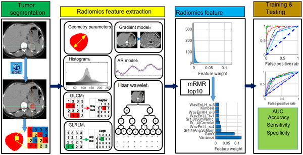
The E3D software (e3d-med.com) was used for marking the region of interest (ROI) (18). The ROI was contoured by experienced physicians at our hospital. The texture features of ROI were then extracted, digitalized, and quantified in MaZda software according to its manual (19-21). Briefly, 352 features were drawn from seven categories (Appendix 1), which were as follows: Autoregressive model (AR model, including coefficients of neighboring pixels, reflecting coarse-to-fine stratification), geometric parameters (GP, including the characteristics of ROI, such as location, orientation, size, and geometric and topological descriptors), gradient model (GM, a direction which changes in the grayscale intensity, representing the image intensity distribution), gray-level co-occurrence matrix (GLCM, computed from the intensities of pairs of pixels, describing homogeneity), gray-level run-length matrix (GLRLM, calculated in four directions, that is, horizontal, vertical, 45°, and 135° angles, indicating image coarseness), the Haar wavelet (HW, spatial frequencies at multiple scales, identifying coarseness), and grayscale histogram (GH, including characteristics reflecting image uniformity). All features were normalized by the 3-sigma method. Next, the weight of each feature was evaluated by the minimum redundancy-maximum relevance (mRMR) algorithm (22), and the top 10 weight features were selected to train and test the diagnostic ML models (Figure 1).
The experimental design and workflow of the study

3.4. Diagnostic ML Models
The training and testing of ML models were performed in Python 3.7, using the Scikit-learn package (23). The following supervised ML algorithms were used with default parameters: AdaBoost classifier, CatBoost classifier, decision tree classifier, extra-trees classifier, extreme gradient boosting, Gaussian process classifier, gradient boosting classifier, k-nearest neighbor classifier, linear discriminant analysis, logistic regression, multi-level perceptron (MLP) classifier, naive Bayes classifier, quadratic discriminant analysis, random forest classifier, ridge classifier, and SVM (linear kernel). All models were run under default parameters (Appendix 2), with a prediction value ≤ 0.5 indicating a benign tumor and > 0.5 indicating RCC. Besides, the performance of the models was evaluated by the receiver operating characteristic (ROC) curve. The accuracy of diagnosis (ACC), sensitivity, and specificity were calculated as follows (24):
where TP represents a true positive, TN represents a true negative, FP represents a false positive, and FN represents a false negative.
4. Results
The age of the patients is presented in Table 1. There was no significant difference in terms of sex or age between the two groups. A total of 5,360 CT images were obtained from 69 patients. The samples were further divided into a training dataset (28 RCC and 20 AML cases; 3,653 CT images) and a testing dataset (12 RCC and 9 AML cases; 1,707 CT images) (Table 1).
The Characteristics and Groups of Patients
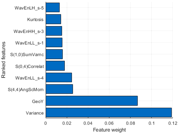
The workflow and strategies applied in this study are presented in Figure 1. Briefly, the CT images were digitized in the E3D software, and the ROI was marked manually. A total of 352 radionics features were extracted in seven categories (Table 2). The weight of each feature was evaluated by the mRMR algorithm (22), and the top 10 features (Figure 2) were selected for the training and testing diagnostic models using 16 supervised ML algorithms. The models were established by the training dataset and validated by the testing dataset. The performance of the models was mainly evaluated by the ROC curve, area under the ROC curve (AUC), and ACC.
Extracted Features for Machine Learning (ML)
| Feature type | Number of features extracted | Number of selected features | Top 10 features | Feature weight |
|---|---|---|---|---|
| Geometric parameters | 73 | 1 | GeoY | 0.0868 |
| Histogram | 9 | 2 | Variance | 0.1188 |
| Kurtosis | 0.0143 | |||
| Gray-level concurrence matrix | 220 | 3 | S(1,0) SumVarnc | 0.0158 |
| S(0,4) Correlat | 0.0177 | |||
| S(4,4) AngScMom | 0.0254 | |||
| Gray-level run-length matrix | 20 | 0 | - | - |
| Gradient model | 5 | 0 | - | - |
| Autoregressive model | 5 | 0 | - | - |
| Haar wavelet | 20 | 4 | WavEnLL_s-1 | 0.0156 |
| WavEnHH_s-3 | 0.0153 | |||
| WavEnHH_s-4 | 0.0245 | |||
| WavEnLH_s-5 | 0.0132 |
Top 10 features for the training and testing diagnostic models. The weight of each feature is calculated by the mRMR algorithm; the top 10 features are selected by weight.

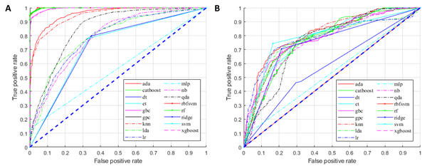
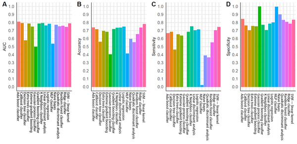
For the training group, all established models, except for the MLP classifier, showed promising performance (Figure 3A). Nonetheless, overfitting was observed, as the AUCs of some models were close to one (Figure 3A). In the testing group, as expected, the models generally had lower AUCs (Figure 3B). However, models built by the AdaBoost classifier, CatBoost classifier, gradient boosting classifier, k-nearest neighbor classifier, linear discriminant analysis, logistic regression, ridge classifier, and SVM (linear kernel) exhibited discriminating potentials for the testing dataset, with AUC of ≥ 0.75 and ACC of ≥ 0.70 (Figure 4A and B).
The receiver operating characteristic (ROC) curves of the training (A) and testing (B) diagnostic models for the diagnosis of renal cell carcinoma (RCC).

Performance of the tested diagnostic models: A, Area under ROC (AUC); B, Accuracy of diagnosis (ACC); C, Sensitivity; and D, Specificity.

In contrast, three models in the testing group, including the decision tree classifier, Gaussian process classifier, and MLP classifier, had AUCs below 0.6 (Figures 3A and 4A), suggesting a poor discrimination power. The SVM model showed the most promising result. Since the AUC values were similar for the tests of training and testing datasets (0.73 and 0.79, respectively), the model had good stability. The ACC of the SVM model (linear kernel) was also the highest in the test (Figure 4). The specificity of the tested models was majorly higher than their sensitivity, and some algorithms with high AUCs had a low ACC (Figure 4); therefore, better performances could be achieved with fine-tuning parameters.
5. Discussion
In this study, 16 algorithms were compared for discriminating RCC from AML. After quantification in MaZda software, 3-sigma normalization, and weight measurement using the mRMR algorithm, the top 10 weight features were fed into all the models with default parameters. Unlike deep learning algorithms, these algorithms showed high explainability, as the main features were clearly defined and carefully selected based on the ranking of weights. Some of the algorithms showed reasonable results based on the AUC of ROC, specificity, and sensitivity analyses. Among all tested algorithms, the SVM (linear kernel) model and AdaBoost classifier yielded the most promising results for the further development of RCC CAD systems.
The SVM algorithm is one of the most common algorithms in CAD development (25, 26). The high prevalence of SVM in our study is consistent with previous research, which found the SVM algorithm to be sensitive for RCC diagnosis (16, 17). In these studies, the AUC of SVM algorithm ranged from 0.8 to 0.9. However, no testing dataset was applied in their models to evaluate overfitting. The present study improved the credibility of SVM algorithm by benchmarking multiple models and applied a carefully designed dataset with properly divided training/testing sets. The AdaBoost classifier had the highest AUC in the testing dataset (Figure 4A). Previous studies have also reported the high AUC of AdaBoost classifier and its potential application in medical imaging processing, particularly in CT imaging (27, 28). However, in the current study, its ACC was only 0.74 due to significant discrepancy between sensitivity and specificity (Figure 4B - D). Therefore, for the AdaBoost classifier, the default threshold setting could not achieve the finest resolution, and more adjustments were required. Research also suggests that the AdaBoost algorithm is sensitive to noise signals, but is less likely to be overfitting; therefore, it is widely tested in ML diagnostic studies (29-31).
Although the results of 16 supervised ML algorithms were different in the present study, each algorithm had its own merits and limitations. The results were greatly influenced by factors, such as data quality, data size, context, feature selection, and manual processing. Therefore, to establish a CAD system that can function in the real world, it is important to compare and examine different strategies repeatedly. Meanwhile, classification of training and testing datasets can greatly affect the results. In the current study, to mimic real-world diagnostics using limited resources, the training and testing sets were divided by patients; therefore, when evaluating the models, the interference of patient-specific factors could be minimized. In our parallel experiment, the training and testing sets were divided by images, which resulted in strong overfitting for many algorithms (Appendix 3). Also, due to the limited number of patients, the characteristics of RCC against AML were not fully recognized by the algorithms. Besides, the relatively small number of patients might have caused bias during model establishment (32).
To reduce the complexity of comparisons, all models in this study were run under a default setting at a cutoff point of 0.5 (0: AML, 1: RCC). Since the present study aimed to perform ML algorithm benchmarking for the diagnosis of RCC, a cutoff point of 0.5 was considered, without any probability threshold optimization. Besides, it should be noted that supervised ML algorithms are original with default parameters, and not all optimization strategies can be considered suitable for the model framework to improve performance. This idea was based on the intuitive concept that the models should be consistently improving in terms of performance. It also suggests the need for further optimization of the current models (e.g., increasing the number of patients, diversifying the source of images, and running models under optimized settings and cutoff points).
Beyond the supervised ML algorithm used in this study, unsupervised ML and deep learning algorithms are being increasingly applied in CAD development to reduce reliance on manual annotation and provide unknown details from radionics (13). The simple experimental design of the current study aimed to provide a baseline benchmarking of 16 algorithms to further indicate the potential application of ML algorithms in CAD systems with highly explainable feature extraction and a rather simple parameter design.
In conclusion, diagnostic classifiers based on ML algorithms for big data were potentially valuable tools for the accurate diagnosis of RCC. The present study suggested candidate algorithms that might show the best performance.
References
-
1.
Liu SZ, Guo LW, Cao XQ, Chen Q, Zhang SK, Zhang M, et al. [Estimation on the incidence and mortality of kidney cancer in China, in 2014]. Zhonghua Liu Xing Bing Xue Za Zhi. 2018;39(10):1346-50. Chinese. [PubMed ID: 30453435]. https://doi.org/10.3760/cma.j.issn.0254-6450.2018.10.011.
-
2.
Xu C, Wang Y, Yang H, Hou J, Sun L, Zhang X, et al. Association Between Cancer Incidence and Mortality in Web-Based Data in China: Infodemiology Study. J Med Internet Res. 2019;21(1). e10677. [PubMed ID: 30694203]. [PubMed Central ID: PMC6371071]. https://doi.org/10.2196/10677.
-
3.
Motzer RJ, Agarwal N, Beard C, Bolger GB, Boston B, Carducci MA, et al. Kidney cancer: Clinical practice guidelines in oncology. J Natl Compr Canc Netw. 2009;7(6):618-30. [PubMed ID: 19555584]. https://doi.org/10.6004/jnccn.2009.0043.
-
4.
Jeon HG, Seo SI, Jeong BC, Jeon SS, Lee HM, Choi HY, et al. Percutaneous Kidney Biopsy for a Small Renal Mass: A Critical Appraisal of Results. J Urol. 2016;195(3):568-73. [PubMed ID: 26410732]. https://doi.org/10.1016/j.juro.2015.09.073.
-
5.
Veltri A, Garetto I, Tosetti I, Busso M, Volpe A, Pacchioni D, et al. Diagnostic accuracy and clinical impact of imaging-guided needle biopsy of renal masses. Retrospective analysis on 150 cases. Eur Radiol. 2011;21(2):393-401. [PubMed ID: 20809129]. https://doi.org/10.1007/s00330-010-1938-9.
-
6.
Ng CS, Wood CG, Silverman PM, Tannir NM, Tamboli P, Sandler CM. Renal cell carcinoma: diagnosis, staging, and surveillance. AJR Am J Roentgenol. 2008;191(4):1220-32. [PubMed ID: 18806169]. https://doi.org/10.2214/AJR.07.3568.
-
7.
Krajewski KM, Pedrosa I. Imaging Advances in the Management of Kidney Cancer. J Clin Oncol. 2018;36(6):3582-90. [PubMed ID: 30372386]. [PubMed Central ID: PMC6299343]. https://doi.org/10.1200/JCO.2018.79.1236.
-
8.
Chow WH, Devesa SS, Warren JL, Fraumeni Jr JF. Rising incidence of renal cell cancer in the United States. JAMA. 1999;281(17):1628-31. [PubMed ID: 10235157]. https://doi.org/10.1001/jama.281.17.1628.
-
9.
Vos N, Oyen R. Renal Angiomyolipoma: The Good, the Bad, and the Ugly. J Belg Soc Radiol. 2018;102(1):41. [PubMed ID: 30039053]. [PubMed Central ID: PMC6032655]. https://doi.org/10.5334/jbsr.1536.
-
10.
Kutikov A, Fossett LK, Ramchandani P, Tomaszewski JE, Siegelman ES, Banner MP, et al. Incidence of benign pathologic findings at partial nephrectomy for solitary renal mass presumed to be renal cell carcinoma on preoperative imaging. Urology. 2006;68(4):737-40. [PubMed ID: 17070344]. https://doi.org/10.1016/j.urology.2006.04.011.
-
11.
Johnson DC, Vukina J, Smith AB, Meyer AM, Wheeler SB, Kuo TM, et al. Preoperatively misclassified, surgically removed benign renal masses: a systematic review of surgical series and United States population level burden estimate. J Urol. 2015;193(1):30-5. [PubMed ID: 25072182]. https://doi.org/10.1016/j.juro.2014.07.102.
-
12.
Canvasser NE, Kay FU, Xi Y, Pinho DF, Costa D, de Leon AD, et al. Diagnostic Accuracy of Multiparametric Magnetic Resonance Imaging to Identify Clear Cell Renal Cell Carcinoma in cT1a Renal Masses. J Urol. 2017;198(4):780-6. [PubMed ID: 28457802]. [PubMed Central ID: PMC5972826]. https://doi.org/10.1016/j.juro.2017.04.089.
-
13.
Langs G, Rohrich S, Hofmanninger J, Prayer F, Pan J, Herold C, et al. Machine learning: from radiomics to discovery and routine. Radiologe. 2018;58(Suppl 1):1-6. [PubMed ID: 29922965]. [PubMed Central ID: PMC6244522]. https://doi.org/10.1007/s00117-018-0407-3.
-
14.
Shen D, Wu G, Suk HI. Deep Learning in Medical Image Analysis. Annu Rev Biomed Eng. 2017;19:221-48. [PubMed ID: 28301734]. [PubMed Central ID: PMC5479722]. https://doi.org/10.1146/annurev-bioeng-071516-044442.
-
15.
Huang S, Yang J, Fong S, Zhao Q. Artificial intelligence in cancer diagnosis and prognosis: Opportunities and challenges. Cancer Lett. 2020;471:61-71. [PubMed ID: 31830558]. https://doi.org/10.1016/j.canlet.2019.12.007.
-
16.
Yu H, Scalera J, Khalid M, Touret AS, Bloch N, Li B, et al. Texture analysis as a radiomic marker for differentiating renal tumors. Abdom Radiol (NY). 2017;42(10):2470-8. [PubMed ID: 28421244]. https://doi.org/10.1007/s00261-017-1144-1.
-
17.
Feng Z, Rong P, Cao P, Zhou Q, Zhu W, Yan Z, et al. Machine learning-based quantitative texture analysis of CT images of small renal masses: Differentiation of angiomyolipoma without visible fat from renal cell carcinoma. Eur Radiol. 2018;28(4):1625-33. [PubMed ID: 29134348]. https://doi.org/10.1007/s00330-017-5118-z.
-
18.
Liu S, He JL, Liao SH. Automatic Detection of Anatomical Landmarks on Geometric Mesh Data using Deep Semantic Segmentation. IEEE International Conference on Multimedia and Expo (ICME). 6-10 July 2020; London, UK. IEEE; 2020.
-
19.
Szczypiński PM, Strzelecki M, Materka A, Klepaczko A. MaZda – The Software Package for Textural Analysis of Biomedical Images. In: Kącki E, Rudnicki M, Stempczyńska J, editors. Computers in Medical Activity, Advances in Intelligent and Soft Computing. Berlin, Germany: Springer; 2009. p. 73-84.
-
20.
Strzelecki M, Szczypinski P. MaZda User's Manual. Lodz, Poland: Institute of Electronics Lodz University of Technology; 1998, [cited 2022]. Available from: http://www.eletel.p.lodz.pl/mazda/download/mazda_manual.pdf.
-
21.
Szczypiński PM, Klepaczko A. MaZda – A Framework for Biomedical Image Texture Analysis and Data Exploration. In: Depeursinge A, Al-Kadi OS, Ross Mitchell J, editors. Biomedical Texture Analysis: Fundamentals, Tools and Challenges. London: Academic Press; 2017. p. 315-47. https://doi.org/10.1016/b978-0-12-812133-7.00011-9.
-
22.
Ding C, Peng H. Minimum redundancy feature selection from microarray gene expression data. Computational Systems Bioinformatics. CSB2003. Proceedings of the 2003 IEEE Bioinformatics Conference. CSB2003. 11-14 August 2003; Stanford, CA, USA. IEEE; 2003. p. 523-8.
-
23.
Moazemi S, Khurshid Z, Erle A, Lutje S, Essler M, Schultz T, et al. Machine Learning Facilitates Hotspot Classification in PSMA-PET/CT with Nuclear Medicine Specialist Accuracy. Diagnostics (Basel). 2020;10(9):622. [PubMed ID: 32842599]. [PubMed Central ID: PMC7555620]. https://doi.org/10.3390/diagnostics10090622.
-
24.
Bradley AP. The use of the area under the ROC curve in the evaluation of machine learning algorithms. Pattern Recognit. 1997;30(7):1145-59. https://doi.org/10.1016/s0031-3203(96)00142-2.
-
25.
Akay MF. Support vector machines combined with feature selection for breast cancer diagnosis. Expert Syst. Appl. 2009;36(2):3240-7. https://doi.org/10.1016/j.eswa.2008.01.009.
-
26.
Peng X, Lin P, Zhang T, Wang J. Extreme learning machine-based classification of ADHD using brain structural MRI data. PLoS One. 2013;8(11). e79476. [PubMed ID: 24260229]. [PubMed Central ID: PMC3834213]. https://doi.org/10.1371/journal.pone.0079476.
-
27.
Ochs RA, Goldin JG, Abtin F, Kim HJ, Brown K, Batra P, et al. Automated classification of lung bronchovascular anatomy in CT using AdaBoost. Med Image Anal. 2007;11(3):315-24. [PubMed ID: 17482500]. [PubMed Central ID: PMC2041873]. https://doi.org/10.1016/j.media.2007.03.004.
-
28.
Nitta T, Muro R, Shimizu Y, Nitta S, Oda H, Ohte Y, et al. The thymic cortical epithelium determines the TCR repertoire of IL-17-producing gammadeltaT cells. EMBO Rep. 2015;16(5):638-53. [PubMed ID: 25770130]. [PubMed Central ID: PMC4428049]. https://doi.org/10.15252/embr.201540096.
-
29.
Xu T, Kim E, Huang X. Adjustable adaboost classifier and pyramid features for image-based cervical cancer diagnosis. IEEE 12th International Symposium on Biomedical Imaging (ISBI). 16-19 April 2015; Brooklyn, NY, USA. IEEE; 2015. p. 281-5.
-
30.
Schapire RE. Explaining AdaBoost. In: Schölkopf BLZVV, editor. Empirical Inference: Festschrift in Honor of Vladimir N. Vapnik. Berlin, Heidelberg: Springer; 2013. p. 37-52. https://doi.org/10.1007/978-3-642-41136-6_5.
-
31.
Hastie T, Rosset S, Zhu J, Zou H. Multi-class AdaBoost. Stat Interface. 2009;2(3):349-60. https://doi.org/10.4310/SII.2009.v2.n3.a8.
-
32.
Byrd RH, Chin GM, Nocedal J, Wu Y. Sample size selection in optimization methods for machine learning. Math Program. 2012;134(1):127-55. https://doi.org/10.1007/s10107-012-0572-5.