

1. Background
Breast cancer is the leading cause of death among women. Two types of abnormal cells are found in the breast: Benign and malignant. Due to the prevalence of thick and fatty tissue and the low ratio of malignant to benign cells, detecting malignant tumors is very challenging (1, 2). Classical methods for diagnosing breast cancer depend on human expertise, resulting in significant labor, time, and susceptibility to human error. Physicians use a standard system known as the breast imaging reporting and data system (BI-RADS) to communicate the findings and results of mammograms, categorizing results into groups numbered 0 through 6 (3).
Artificial intelligence (AI) algorithms can serve as appropriate models to assist physicians in diagnosing breast cancer and categorizing patients. The integration of AI in the field of medical science is of paramount importance for improving the accuracy and performance of disease diagnosis (4-6). Promising reports on machine learning (ML) methods and intelligent techniques in breast cancer diagnosis research indicate their potential to enhance diagnostic performance (7, 8). In recent years, various ML techniques have been applied to the diagnosis and classification of breast cancer to distinguish between malignant and benign cases.
Dutta et al. (9) introduced a classification approach for data mining in medicine. The approach applied an improved fireworks optimization algorithm with the best selection strategy (IFWABS) in the multilayer neural network. The IFWABS approach was tested on the Wisconsin Diagnostic Breast Cancer (WDBC) dataset, resulting in a testing accuracy of 96.98%.
Dora et al. (10) suggested a novel classification approach based on the Gauss-Newton method and sparse representation technique (GNRBA) for breast cancer diagnosis. The efficiency of the GNRBA approach was examined on the UCI WDBC dataset, resulting in a classification accuracy of 98.48%.
Saygili (11) conducted research on several classification methods for breast cancer, and the best accuracy was obtained by the multi-layer perceptron (MLP) neural network technique (98.41%). Jafari-Marandi et al. (12) offered a novel breast cancer diagnosis approach based on a life-sensitive method, a self-organizing map neural network, and an error-driven learning model (LS-SOED). This method employed a decision-oriented neural network based on hybrid supervised and unsupervised learning. The resulting classification accuracy of LS-SOED was 96.19% based on the WDBC dataset.
Wang et al. (13) suggested a novel breast cancer classification method applying the support vector machine based on weighted area under the curve and ensemble learning model (WAUCE). The simulation outcomes revealed that WAUCE achieved a 98.76% accuracy. Rao et al. (14) developed a new method based on the coherently integrated artificial bee colony optimization algorithm and gradient boosting decision tree technique (ABCODT) to select optimal feature subsets. Several UCI datasets, including the WDBC dataset, were subjected to the ABCODT approach. Tests were carried out using the WDBC dataset, resulting in a classification accuracy of 97.18%.
Liu et al. (15) employed a new hybrid technique for breast cancer detection. The information gain method, simulated annealing algorithm, and genetic wrapper approach (IGSAGAW) were used to select optimal features, and a support vector machine based on cost-sensitive (CSSVM) was used as a classifier in this hybrid technique (IGSAGAW-CSSVM). The results of experiments on the UCI-WDBC dataset demonstrated a classification accuracy of 95.7%.
Lu et al. (16) proposed a novel breast cancer classification method using a genetic optimization algorithm and an online gradient boosting model (GAOGB). On the WDBC dataset, the GAOGB method achieved a classification accuracy of 94.51%. Abdar et al. (17) presented a novel breast cancer diagnosis method by utilizing a two-layer nested ensemble model based on stacking and voting ensemble techniques and Naïve Bayes classifier (SV-Naïve-Bayes). The presented method achieved a classification accuracy of 98.07% when applied to the UCI WDBC dataset.
Dalwinder et al. (18) suggested a new breast cancer classification approach using a feature weighting technique based on the ant lion optimization algorithm and a multilayer neural network classifier (FW-BPNN). The approach was tested on the WDBC dataset, resulting in a classification accuracy of 99.3%. Kumar et al. (19) presented a novel medical data classification using genetic programming (GP) based on a new fitness function. The presented technique was applied to the WDBC dataset and achieved an accuracy of 97.69%.
Sahebi et al. (20) developed a new generalized wrapper feature selection (FS) technique based on a new parallel genetic approach (GeFeS). The performance of the GeFeS approach was evaluated using the k-nearest neighbor (KNN) classifier. Experiments conducted with the WDBC dataset demonstrated an accuracy of 98.51% for classification.
Khandezamin et al. (21) introduced a novel hybrid method for breast cancer detection. An FS algorithm based on logistic regression and a new deep neural network dubbed group method data handling (GMDH) were used in the hybrid technique. The experimental results demonstrated that the GMDH method achieved an accuracy of 99.6% on the WDBC dataset.
Kalagotla et al. (22) presented a new method using FS based on correlation and AdaBoost techniques, along with a novel stacking technique with multi-layer perceptron, support vector machine, and logistic regression (Stacking). The method was tested on the WDBC dataset, and the classification accuracy was 97.4%. Wan et al. (23) developed a new hybrid FS approach considering feature interaction based on neighborhood rough set-based information theory (NCMI-IFS). The performance analysis was executed on the WDBC dataset and achieved a classification accuracy of 98.03%.
Although the performance of breast cancer detection highly depends on classification accuracy, most good classification methods have a fundamental flaw: They seek to maximize classification accuracy while ignoring the costs of misclassification among various categories. Based on our experience, the risk of missing a breast cancer case is unquestionably greater than the cost of mislabeling a benign case. Moreover, methods tend to overfit the data, resulting in poor generalization and high computational costs. Therefore, to increase classification performance and lower costs, it is crucial to explore a subset of efficient and optimal features while avoiding overfitting. The primary concept of FS is to choose a subset of variables that can significantly improve the time complexity and accuracy of a classification model. This is particularly important in classification problems when the initial set of features is large. With such a large number of features, it is of special interest to search for a dependency between the optimal number of selected features and the accuracy of the classification model. Therefore, it is critical for researchers to develop an effective algorithm, especially given the high cost of misdiagnosis in breast cancer diagnosis.
To carefully avoid overfitting and determine the relevance of features and class, this study proposes a novel hybrid approach that is more accurate and intelligent. The proposed approach significantly improves breast cancer classification performance and reduces the cost of misclassification. This approach employs a grey wolf optimization algorithm and a self-organizing fuzzy logic classifier (GWO-SOF) to accurately classify breast cancer data. The performance of the approach was evaluated on the WDBC dataset.
Grey wolf optimization, as a metaheuristic swarm intelligence algorithm, can provide the optimal trade-off between local search and global search. This algorithm has characteristics that are flexible, simple, and scalable, leading to favorable convergence. In addition, the SOF classifier is highly objective and non-parametric. This implies that data are not subjected to any generating model with parameters, and without any prior information and knowledge about the problems, all associated meta-parameters are immediately obtained from data. Therefore, the SOF is a highly adaptable classifier that has demonstrated excellent performance on a range of problems. On the other hand, the quality of the selection metrics and techniques has a significant impact on the performance of learning models that use the FS process. The GWO and the SOF have many inherent advantages that can be summarized as follows:
The GWO algorithm offers an optimal trade-off between local search and global search.
The GWO algorithm has the advantages of having fewer control parameters and favorable convergence.
The SOF classifier is highly objective and non-parametric.
The SOF classifier is a highly adaptable classifier.
This work hybridizes the BGWO algorithm and the SOF classifier to validate the supervised learning model effectively. The BGWO-SOF hybrid approach efficiently removes unimportant features from the feature space and generates an optimal feature subset while preserving the latent structure of the dataset.
2. Methods
In this section, the materials and methods applied in the proposed approach are described. First, the breast cancer dataset used in this work is introduced. Then, the GWO and SOF classifiers are explained. Finally, the proposed approach is presented.
2.1. Dataset
The WDBC dataset was obtained from the UCI Machine Learning Repository and utilized in this work (24). This dataset is frequently used in medical and breast cancer studies to evaluate ML approaches, including classification and FS. The tumor features in the WDBC dataset were extracted from digital images of fine needle aspirates (FNAs) of breast masses, describing characteristics of cell nuclei present in the images. The WDBC dataset comprises 32 features collected from 569 individuals, including (a) an instance ID number, (b) 30 real-valued features computed for each cell nucleus, and (c) a class attribute indicating benign or malignant cases. Each instance has 10 cell nuclei properties measured, and various statistics of these 10 attributes are computed, such as mean, standard error, and maximum, resulting in a total of 30 features, as shown in Table 1. The dataset is distributed with 37.25% and 62.75% benign and malignant instances, respectively.
| Attribute Number | Attributes | Comment | Attributes Range | ||
|---|---|---|---|---|---|
| Mean | Standard Error | Specificity | |||
| 1 | Radius | Mean of distances from the center to points on the perimeter | 6.98 - 28.11 | 0.112 - 2.873 | 7.93 – 36.04 |
| 2 | Texture | The standard deviation of gray-scale values | 9.71 - 39.28 | 0.36 - 4.89 | 12.02 – 49.54 |
| 3 | Perimeter | 43.79 - 188.50 | 0.76 - 21.98 | 50.41 – 251.20 | |
| 4 | Area | 143.50 – 2501.00 | 6.80 – 542.20 | 185.20 – 4254.00 | |
| 5 | Smoothness | Local variation in radius lengths | 0.053 – 0.163 | 0.002 – 0.031 | 0.071 – 0.223 |
| 6 | Compactness | Perimeter2 / area - 1.0 | 0.019 – 0.345 | 0.002 – 0.135 | 0.027 – 1.058 |
| 7 | Concavity | Severity of concave portions of the contour | 0.000 – 0.427 | 0.000 – 0.396 | 0.000 – 1.252 |
| 8 | Concave point | Number of concave portions of the contour | 0.000 – 0.201 | 0.000 – 0.053 | 0.000 – 0.291 |
| 9 | Symmetry | 0.106 – 0.304 | 0.008 – 0.079 | 0.157 – 0.664 | |
| 10 | Fractal dimension | “Coastline approximation” - 1 | 0.050 – 0.097 | 0.001 – 0.030 | 0.055 – 0.208 |
Description of the Wisconsin Diagnostic Breast Cancer (WDBC) Dataset
2.2. Feature Selection
Machine learning employs methods that allow the analysis of large amounts of data automatically (25). Classification algorithms are a type of supervised learning technique used to identify the category of new observations based on training data. In classification, a program learns from a given dataset and then classifies new observations into predefined classes. The primary objective of classification is to generalize from the training patterns to accurately categorize new patterns. The process of ML for classification begins with prerequisites, such as datasets, data cleaning procedures, FS techniques, and classification models (26-28).
Feature selection is a crucial aspect of ML. Feature selection techniques for classification problems are based on identifying significant features, and these techniques can enhance various standard ML methods (29, 30). Therefore, this process plays a vital role in the development of learning models. Selecting the appropriate and optimal feature subset can be challenging due to the complex and unpredictable interrelationships between features (31, 32). Since FS is a near-optimal (NP)-hard problem (33, 34), several optimization algorithms have been proposed to overcome its limitations. These algorithms include particle swarm optimization (PSO) (35, 36), ant colony optimization (ACO) (37, 38), whale optimization (WO) (39, 40), and GWO (41). Feature selection approaches based on optimization algorithms have the ability to efficiently explore large search spaces and often yield results that closely approximate the global solution. These approaches systematically eliminate unnecessary and redundant features, which can, in many cases, enhance the performance of learning models by reducing uncertainty and overfitting issues (42-44).
2.3. Grey Wolf Optimization Algorithm
Optimization algorithms refer to procedures for finding near-optimal solutions to multi-dimensional and complex optimization problems. One such optimization algorithm is the GWO algorithm. The GWO algorithm is a promising optimization technique based on swarm intelligence (SI) (45). This algorithm has garnered the attention of many researchers across various optimization domains (46-48). What sets the GWO algorithm apart from other evolutionary and swarm intelligence techniques are its distinctive characteristics. The GWO algorithm requires minimal parameter tuning, effectively balances global and local search, and demonstrates favorable convergence. Moreover, it is known for its simplicity of implementation, adaptability, and scalability (49).
The GWO algorithm mimics the natural hierarchy of leadership and hunting mechanisms observed in grey wolves. It employs four types of grey wolves to simulate the hierarchy of leadership: Alpha (α), beta (β), delta (δ), and omega (ω). Grey wolves tend to live in herds and group environments, with group sizes ranging from a minimum of 5 to a maximum of 12. The hierarchy among grey wolves is highly structured, with α representing the best outcome in mathematical terms, followed by β and δ as the next level of preferred outcomes. The ω outcome is another consideration. The GWO algorithm posits that α, β, and δ wolves lead the hunt (optimization); however, ω wolves monitor these three leaders (45). The crucial phase of the hunt occurs when a wolf encircles its prey. Equations are employed to represent the encircling behavior of the GWO algorithm.
Where D_i is calculated in Equation the current iteration is defined as t; p and y are positions of prey and grey wolves, respectively.
Where A and C are coefficient vectors that are determined using Equations
Where r1 and r2 are random vectors in the range of [0, 1], and the lb components are linearly lowered from 2 to 0. The hunting process is frequently directed by α. Grey wolves, both β and δ, sporadically attend the hunt. However, the exact position of the best solution (prey) in the problem’s abstract search space is unknown. Therefore, it was believed that α would be the best potential solution for the simulation of wolf hunting behavior; nevertheless, β and δ would present a better understanding of where the prey could be found. As a result, the top three findings obtained were set reserved. Omegas and other search agents must change their positions to the best search agents’ positions. Equation is utilized to update the positions of wolves.
Where W1, W2, and W3 are formulated in Equations to 8, accordingly.
Where Wα, Wβ, and Wδ are the GWO’s first three most effective solutions at a certain iteration t, A1, A2, and A3 are defined in Equation and Diα, Diβ, and Diδ are formulated in Equations to 11, accordingly.
where C1, C2, and C3 are formulated in Equation Finally, according to Equation the parameter lb was reduced (2 - 0) to emphasize global and local search.
Where t denotes the current number of iterations, and Maxit denotes the maximum iterations permitted in the GWO.
2.4. Binary GWO
The binary GWO algorithm has been called BGWO, where each solution contains a combination of 0's and 1's. Emary et al. proposed a new BGWO algorithm applied for FS tasks (50). In this algorithm, the wolves that updated the equation represented a three-position vector function: Wα, Wβ, and Wδ, which were in charge of inviting each of the wolves to the best three outcomes. The position of a specific wolf is included using the GWO principle while maintaining the binary constraint according to Equation The scholars employed the update on the GWO method, which is detailed in Equations to 23. The core update equation is expressed in Equation
Where w1, w2, and w3 binary vectors reflect the influence of a wolf’s movement toward α, β, and δ grey wolves in order. w1, w2, and w3 vectors are computed by Equations and 20, respectively.
where
where urand is a random number generated from a standard uniform distribution in the range (0,1), and
where
where
where urand is a random number generated from a standard uniform distribution in the range (0,1), and
where
where
where urand is a random number generated from a standard uniform distribution in the range (0,1), and
where
2.5. Self-Organizing Fuzzy Logic
Gu et and Angelov introduced a novel classifier model based on SOF (51). The SOF classifier utilizes non-parametric statistical operators to objectively reveal essential data patterns, even in the absence of empirically acquired data samples. It identifies local peaks within the multi-modal data distribution to serve as prototypes. Additionally, the SOF classifier is highly objective and non-parametric. This means that it does not rely on a predefined model with parameters. Instead, it derives all associated meta-parameters directly from the data itself. Depending on the complexity of the problem and the availability of computational resources, the SOF classifier can address issues at various levels of granularity or detail. Furthermore, it supports both online and offline learning and can classify data using various dissimilarity/distance criteria. Therefore, the SOF is a versatile classifier known for its excellent performance across a range of problems. In this paper, the offline learning mode of the SOF classifier will be utilized.
The SOF classifier’s offline method involves independently detecting prototypes for each class and constructing a zero-order fuzzy rule of the AnYa type based on the identified prototypes for each class (in the structure of Equation
The AnYa-type fuzzy rule-based scheme was introduced in (52) as an alternative approach to the commonly used fuzzy rule-based schemes, such as Takagi-Sugeno (53) or Mamdani (54) models. In comparison to the two previous models, the pattern component (IF) in AnYa-type fuzzy rules is streamlined into a more concise, objective, and non-parametric vector structure without requiring the definition of ad-hoc membership functions, as needed in the two aforementioned predecessors. The following is the form of a zero-order fuzzy rule of the AnYa type:
Where xin signifies vector of input and “∼” signifies similarity, which can also be considered a fuzzy degree of membership/satisfaction (55); proi (i=1,2,..., Np) represents the class’s ith prototype; Np is the number of prototypes discovered from the data samples of this class. Different strategies, such as “fuzzily weighted average”, might be used to determine the label for a specific data sample.
The fuzzy rule training procedures of separate classes will have no effect on each other. We will suppose for the remainder of this section that the training procedure is conducted using data samples from the cth class (c=1,2,..., C) indicated by
Prototypes are found using the densities and mutual distributions of data samples in the method. To begin with, multi-modal densities
By discovering the sample of data with the largest multi-modal density,
The entire list{r} is built by repeating the procedure until each of the data samples has been chosen, and based on the list{r}, the multi-modal densities of
It is important to note that after a data sample is selected into list{r}, it cannot be selected for a second time.
Prototypes, indicated by {p}0 are then
recognized as the local maximum of the ordered multi-modal densities,
Condition 1:
After all of the prototypes have been recognized with Equation some fewer representative ones might be found in {p}0, thereby necessitating the use of a filtering process to eliminate them from P0.
Before beginning the filtering process, use the prototypes to attract close data samples to construct data clouds (55), similar to Voronoi tessellation (58):
After all the clouds of data are generated around the available prototypes {p}0, one can acquire the data cloud centers Indicated by {φ}0, and the multi-modal densities at the centers are computed by
Following that, for each data cloud, supposing the ith one
Condition 2:
Where
Condition 3:
In the end, the representative prototypes of the cth class {p}c are recognized, the fuzzy rule of AnYa type might be constructed as follows, where Nc denotes the number of prototypes in {p}c:
2.6. The Hybrid Intelligent Method
Taking into consideration the advantages of BGWO and SOF and the importance of breast cancer classification, this study proposes an intelligent approach for distinguishing benign from malignant breast cancers. In the proposed approach, BGWO acts as an FS technique to select the effective and optimal features; nevertheless, SOF functions as the classifier to evaluate the performance of these optimal features. The procedure of the proposed approach (BGWO-SOF) is described below.
The procedure begins with normalizing the values of the WDBC dataset and initializing the parameters for the BGWO algorithm. Then, the K-fold cross-validation technique is employed (with K = 10) to assess how effectively the classification approach can predict the tumor characteristics of an unknown instance. For each fold, the dataset is divided into 10 equally sized subsets. Consequently, in each fold, 9 subsets serve as the training data (90% of the dataset); however, 1 subset (10% of the dataset) is reserved for testing purposes.
In each fold, the algorithm executes the optimization process by generating an initial population of candidate solutions (i.e., individuals) within the search space. Each position of an individual is represented as a vector with N elements, where N is the number of features in the dataset. A 0 value indicates that a certain feature is not selected; nonetheless, a 1 value indicates that the related feature is selected. Each individual in the feature space constitutes a set of candidate features. The BGWO solution is depicted in Figure 1 (for example, N = 10).

Solution representation of feature selection
Then, the fitness for each solution (𝑋𝑖) is calculated. Because the approach’s primary goal is to improve the performance of the classification, the quality of a solution is determined by two key criteria: The number of BGWO-selected features in the solution and the SOF classifier’s error rate. Therefore, the optimal solution is a combination of features with the fewest number of selected features and the highest performance of classification. In this paper, the fitness function in Equation by the SOF classifier is applied to evaluate the quality of the features selected by the BGWO.
Where
At each iteration, the fitness or classification error rate of the new solution is compared to the fitness of the previous solution, and if it shows an improvement, the new solution is chosen. The process is repeated until the total number of iterations reaches a certain limit called Maxit. Finally, the sets of the selected features are used in the SOF learning model.
This procedure will be repeated until all of these subsets apply for both the training and testing phases. Finally, the evaluation metrics results from the 10 iterations are averaged to produce reliable statistical results. Figure 2 shows a flowchart of the proposed approach.

Flowchart of the proposed approach
3. Results
This section presents the experimental setup, including the dataset and parameter settings, evaluation metrics, and details of the experiment’s execution and results analysis, to verify and examine the performance of the proposed approach.
3.1. Experimental and Parameter Settings
This study evaluated the performance of BGWO-SOF using the WDBC breast cancer dataset. For the experimental executions, this study utilized an Intel(R) Core (TM) i5 CPU 8250U 1.6GHz with 8 GB of RAM, running MATLAB 2018 on a Windows 10 (64-bit) operating system. The BGWO-SOF was executed with a population size of 20. The approach was formulated as an optimization problem, and BGWO was run for 50 iterations. In the SOF classifier, the Euclidean distance was employed as a dissimilarity metric with a granularity level equal to 12. To prepare for experimentation, the values from the WDBC dataset were normalized. Subsequently, a 10-fold cross-validation technique was employed to assess the performance of the proposed approach.
3.2 Evaluation Metrics
This work focused on a two-class classification problem, where a classifier produces two discrete results: Negative and positive. The experiments were conducted on the WDBC dataset, resulting in four possible outcomes in the confusion matrix, as shown in Figure 3. When a positive instance is correctly classified as positive, it is a true positive (TP). Conversely, a false negative (FN) occurs when a positive instance is incorrectly classified as negative. Similarly, when a negative instance is correctly classified as negative, it is a true negative (TN); however, an incorrect classification of a negative instance as positive is a false positive (FP).

Confusion matrix in a two-class classification
In the WDBC dataset, patient instances with benign tumors are labeled as 0 (negatives); however, those with malignant tumors are labeled as 1 (positives). True negatives are instances where the actual class was negative, and the expected class was also negative. True positives are instances with a positive current class and a positive expected class. False negatives occur when a record’s true class is positive but is expected to be negative; nevertheless, FPs occur when the record’s actual class is negative; nonetheless, the expected class is positive. When dealing with cancer diagnosis results, minimizing FNs is crucial.
This study employed classification performance metrics, including accuracy, precision, recall (also known as sensitivity), F-measure, Matthews correlation coefficient (MCC), and specificity, for the evaluation and comparison of the proposed approach on the WDBC dataset. Accuracy measures the percentage of times a classifier produces correct results. The precision determines how accurately a classifier predicts a positive pattern (yes). Recall, also known as sensitivity or true positive rate, indicates how well a classifier predicts a pattern’s identity. Specificity measures the frequency at which a classifier predicts non-patterns (no). The F-Measure is the harmonic average of recall and precision. Matthews correlation coefficient assesses the quality of binary classifications and is a more reliable statistical rate than balanced accuracy. It produces a high score only if the prediction performs well in all four confusion matrix categories in proportion to both the size of positive and negative elements in the dataset. The following formulas are used to calculate the evaluation metrics:
The trade-off between the FP rate (1-specificity) and the TP rate (sensitivity) is depicted by a receiver operating characteristic curve (ROC curve). The ROC curve is a graphical diagram that illustrates how the diagnostic capacity of a binary classifier system changes with its discrimination threshold. Classifiers that yield curves closer to the top-left corner indicate better performance. The ROC curve does not depend on the class distribution, making it useful for evaluating classifiers predicting rare events.
3.3. Experimental Results
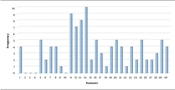
The first experiment evaluates the performance of the present proposed approach (BGWO-SOF) and the SOF classifier without feature selection capability (SOF-WFS). The classification ability of the method is assessed using 10-fold cross-validation. Table 2 shows the experimental results as the average of the 10-fold cross-validation outcomes. Table 2 shows that by using BGWO-SOF, classification accuracy, and other metrics have improved dramatically, with the BGWO-SOF approach outperforming the SOF-WFS method. The average accuracy for the SOF method was 80.54%; however, the best accuracy for BGWO-SOF is 99.702%; nevertheless, the number of features was reduced by approximately 64%. Since the 10-fold cross-validation method was applied in this study, the ROC curve is generated from 10 folds. Figure 4 illustrates the ROC curve for the 10 folds, demonstrating the classifier’s efficiency and its capability to distinguish between classes. Figure 5 presents the number of selected features by the proposed approach in each iteration. The proposed approach selects the best and optimal subset of features, reducing the feature count by 62% in the FS process. Figure 6 indicates the frequencies of the selected features using the BGWO-SOF approach on the WDBC dataset over 10 iterations.
| Method | Accuracy | Sensitivity | Specificity | Precision | F-measure | MCC |
|---|---|---|---|---|---|---|
| SOF without feature selection | 80.54 | 85.33 | 72.34 | 80.27 | 82.60 | 78.13 |
| BGWO-SOF (feature selection) | 99.702 | 99.681 | 99.679 | 99.646 | 99.658 | 98.973 |
Experimental Results (%) of Binary Grey Wolf Optimization-Self-Organizing Fuzzy Logic Classifier (BGWO-SOF) and SOF Classifier Without Feature Selection (SOF-WFS) Methods
 curve")
The receiver operating characteristic (ROC) curve

Number of selected features

Frequency of selected features
4. Discussion
In this study, the BGWO algorithm was combined with the SOF classifier to validate the supervised learning model effectively. The BGWO-SOF hybrid approach can efficiently eliminate unimportant features from the feature space and generate an optimal feature subset while capturing the latent structure of the dataset. The quality of the selection metrics and techniques significantly impacts the performance of learning models utilizing the FS process. To demonstrate the effectiveness of the proposed approach, the BGWO-SOF findings (average metric values) were compared to several recently published approaches in the field of FS and breast cancer classification. This study examined articles in the literature that utilized the same dataset (WDBC) and evaluation metrics (8, 12-15, 17-23, 59)
Table 3 shows the results of this comparison. In terms of classification accuracy, the results demonstrated that the proposed approach is more accurate and robust than state-of-the-art methods. Although classification accuracy is highly important for breast cancer detection, many good classification methods have significant drawbacks in that they aim solely to maximize classification accuracy, often ignoring the costs associated with misclassification across different categories. Evaluating a learning model’s performance solely based on classification accuracy might not indicate its superiority. As shown in Table 3, to further assess the likelihood of class imbalance and its impact on accuracy, this study examined metrics such as recall, precision, F-measure, and specificity. The average F-measure value, close to 1 (0.99742), indicates that the proposed approach has a very low number of FP and FN, signifying excellent precision and recall percentages. Additionally, the average MCC value (close to 1) suggests that both classes are predicted effectively. Figure 7 depicts comparisons between the present study’s approach’s results and the findings of previous research. The results demonstrated that the proposed approach outperforms other state-of-the-art methods in all evaluation metrics.
In general, the results of the proposed approach are satisfactory for all the evaluation metrics. The evaluation results indicated that the proposed hybrid approach can not only effectively reduce the feature space dimensions but also ensure the efficiency and acceptable performance of the classification model. The experimental and comparison results for all the evaluation metrics demonstrate that the proposed approach outperforms other well-known methods in classification.
Since we used the standard WDBC dataset for this study, there was no access to the BI-RADS stages of cases in this dataset. Therefore, only two classification levels were considered: Benign and malignant. For future studies, it is recommended to use datasets of real patients with specific tumor grades (BI-RADS) to extract features for each BI-RADS category and evaluate the FS and classification performance for each of them. Furthermore, future studies can include more patient characteristics, such as demographic features, to create more accurate models.
It is important to note that, despite using the WDBC dataset from the UCI Machine Learning Repository, the proposed approach does not have any specific limitations for testing on real datasets. In practice, when using a real dataset, the following operations must be taken into account to ensure a clean dataset:
Features must be extracted from real samples.
Valid samples must be separated, and damaged or invalid samples must be removed.
An expert doctor must classify the data samples as benign or malignant.
| Variables | LS-SOED (12) | WAUCE (13) | ABCoDT (14) | IGSAGAW-CSSVM (15) | GAOGB (8) | SV-Naïve-Bayes (17) | FW-BPNN (18) | GP (19) | GeFeS (20) | GMDH (21) | Stacking (22) | NCMI_IFS (23) | ESO-GSO (59) | BGWO-SOF |
|---|---|---|---|---|---|---|---|---|---|---|---|---|---|---|
| Accuracy | 96.19 | 97.68 | 97.18 | 95.7 | 94.28 | 98.07 | 98.37 | 97.69 | 98.51 | 99.60 | 97.4 | 98.03 | 98.95 | 99.702 |
| Recall | 94.75 | - | - | 93.11 | - | - | 96.03 | 98.1 | 99.53 | 92.5 | - | 96.96 | 99.681 | |
| Specificity | - | 99.49 | - | - | 93.20 | - | - | 97.02 | - | - | - | - | - | 99.679 |
| Precision | - | - | - | - | - | - | 95.03 | 99.3 | 99.53 | 96.2 | - | 100 | 99.646 | |
| F-measure | - | - | - | - | - | - | - | 95.02 | 98.7 | 99.53 | 94.2 | - | 96.96 | 99.658 |
| MCC | - | - | - | - | - | - | - | - | - | - | - | - | - | 98.973 |
Comparison of Results with State-of-the-art Methods
; artificial bee colony and gradient boosting decision tree algorithm (ABCoDT); information gain directed simulated annealing genetic algorithm wrapper (IGSAGAW); cost sensitive support vector machine (CSSVM); genetic algorithm-based online gradient boosting (GAOGB); Back-propagation neural networks (FW-BPNN); genetic programming (GP); generalized feature selection algorithm (GeFeS); group method data handling (GMDH); interaction feature selection algorithm based on neighborhood conditional mutual information (NCMI_IFS); eagle strategy optimization (ESO); gravitational search optimization (GSO); binary grey wolf optimization algorithm and a self-organizing fuzzy logic classifier (BGWO-SOF)")
Accuracy comparison of the proposed approach to state-of-the-art methods (abbreviations: Weighted area under the receiver operating characteristic curve ensemble (WAUCE); artificial bee colony and gradient boosting decision tree algorithm (ABCoDT); information gain directed simulated annealing genetic algorithm wrapper (IGSAGAW); cost sensitive support vector machine (CSSVM); genetic algorithm-based online gradient boosting (GAOGB); Back-propagation neural networks (FW-BPNN); genetic programming (GP); generalized feature selection algorithm (GeFeS); group method data handling (GMDH); interaction feature selection algorithm based on neighborhood conditional mutual information (NCMI_IFS); eagle strategy optimization (ESO); gravitational search optimization (GSO); binary grey wolf optimization algorithm and a self-organizing fuzzy logic classifier (BGWO-SOF)
4.1. Conclusions
Breast cancer ranks among the leading causes of mortality worldwide, particularly among women. This pressing issue has prompted extensive research in the field of medicine. The primary objective of this study was to introduce an intelligent approach to breast cancer detection, with the aim of aiding clinical practitioners in making more informed decisions in the future.
In this paper, we proposed a novel hybrid intelligence approach that combines the GWO algorithm with the SOF classifier. The performance of this hybrid approach was assessed using the WDBC dataset and a stratified 10-fold cross-validation. Various standard performance evaluation metrics, including accuracy, F-measure, precision, sensitivity, and specificity, were employed in the experiments. Upon comparing the results, it was observed that the proposed approach consistently yielded superior or competitive results when compared to other state-of-the-art methods. In the future, it is planned to further develop and expand this approach by incorporating additional optimization algorithms and classification techniques.
