
1. Background
Cardiovascular disease (CVD) remains one of the leading contributors to mortality worldwide (1). Air pollution and meteorological variation can influence cardiovascular risk through inflammatory, oxidative, vascular, and autonomic pathways, and these relationships are particularly relevant in cities where traffic emissions, industrial activity, heat, and dust events can vary over short periods (2). Evidence from Iran and other dry-climate settings has also shown that air pollution and dust-related exposures may be associated with cardiovascular mortality and related health outcomes (3-6).
This study focuses on forecasting rather than causal exposure estimation. Public health teams may need to anticipate short-term cardiovascular mortality patterns even when the causal pathway underlying each daily fluctuation is uncertain. For this task, recent mortality history may be highly informative, whereas environmental variables may add value only when their timing and scale align with the relevant risk processes.
Classical time-series models and recurrent neural networks involve different trade-offs. Autoregressive integrated moving average (ARIMA) provides a transparent baseline for temporal dependence in a univariate mortality series, whereas ARIMA with exogenous variables (ARIMAX) extends this framework by allowing external regressors to enter the forecasting equation (7-9). Recurrent neural networks (RNNs), long short-term memory (LSTM), and gated recurrent unit (GRU) models can learn nonlinear sequential relationships and may be useful when temporal patterns are difficult to represent with a linear specification (10-12). However, their flexibility makes evaluation more demanding: stochastic initialization, hyperparameter choices, validation design, and train-test splitting can alter the apparent ranking.
The broader forecasting literature includes GRU/LSTM comparisons, environmental and health forecasting reviews, ARIMAX and convolutional neural network (CNN)-LSTM mortality forecasting, seasonal ARIMA (SARIMA)/SARIMA with exogenous factors (SARIMAX) and hybrid time-series applications, activation-function studies, and nonlinear pollutant-prediction models (13-23). These studies provide methodological context, whereas the present evaluation was limited to ARIMA, ARIMAX, RNN, LSTM, and GRU.
Environmental variables can be incorporated in several ways. A univariate design tests whether mortality history alone is sufficient for short-term forecasting. A cross-correlation function (CCF)-selected multivariate design assigns each environmental predictor a training-period lag chosen via cross-correlation screening. A manual 7-day multivariate design applies the same 7-day lag to all environmental variables. These are forecasting input designs, not exposure-response models. They assess whether environmental information improves prediction in a particular form; they do not estimate the number of deaths caused by a pollutant.
2. Objectives
This study compared ARIMA, ARIMAX, RNN, LSTM, and GRU models for forecasting daily cardiovascular mortality in Shiraz across three input designs. The primary analysis used an 80/20 chronological split, and a 70/30 chronological split was used as a sensitivity analysis. For recurrent models, the evaluation was seed-aware and combined root mean square error (RMSE)-based ranking with formal statistical tests of mean squared error (MSE) loss to distinguish the lowest observed error from evidence of a statistically distinct winner.
3. Methods
In brief, this study used 10 years of daily cardiovascular mortality and environmental data from Shiraz to compare five forecasting model families—ARIMA, ARIMAX, RNN, LSTM, and GRU—across three input designs: mortality history alone (univariate), environmental predictors at empirically selected lags (CCF-selected multivariate), and environmental predictors at a fixed 7-day lag (manual multivariate). Models were trained on an earlier portion of the time series and evaluated on a chronologically held-out test period. The evaluation combined descriptive error ranking with formal statistical testing to distinguish the lowest observed error from evidence of a statistically superior model. Full technical details are provided in the subsections below.
3.1. Study Design and Data Source
This retrospective daily time-series forecasting study used records from Shiraz, Iran, covering the period from 21 March 2010 to 19 March 2020. Daily cardiovascular mortality counts were obtained from the Health Deputy of Shiraz University of Medical Sciences and included all cardiovascular deaths recorded among Shiraz residents across all age groups and both sexes throughout the study period. Cardiovascular mortality was defined using International Classification of Diseases, 10th Revision (ICD-10) codes I20–I25, I46–I50, R98–R99, and R09.2, encompassing acute myocardial infarction, stroke, hypertensive heart and renal disease, pulmonary embolism, arterial embolism and thrombosis, aortic aneurysm, heart failure, cardiomyopathy, endocarditis, pericarditis, myocarditis, nonrheumatic mitral and aortic valve disorders, and congenital cardiovascular anomalies. The dataset represents population-level registry records for the city of Shiraz; no sampling was applied, and all days within the study period were included.
Candidate environmental predictors included daily concentrations of five criteria air pollutants—carbon monoxide (CO), ozone (O3), nitrogen dioxide (NO2), sulfur dioxide (SO2), and particulate matter with aerodynamic diameter less than 10 μm (PM10)—together with mean temperature and relative humidity. Air pollutant data were obtained from a single air quality monitoring station located in Shiraz. Each pollutant was measured 24 times per day, and the daily mean concentration was calculated across all hourly measurements for each study day. Daily mean temperature and relative humidity were obtained from the Fars Province Meteorological Organization.
Calendar dates were retained for chronological ordering, lag construction, train-test splitting, and sequential model input construction. The study used de-identified, aggregated secondary records. Ethics approval and consent-waiver details are reported in the Declarations section.
Figure 1 shows the study workflow, including preprocessing, input design, model training, and leakage-control steps.
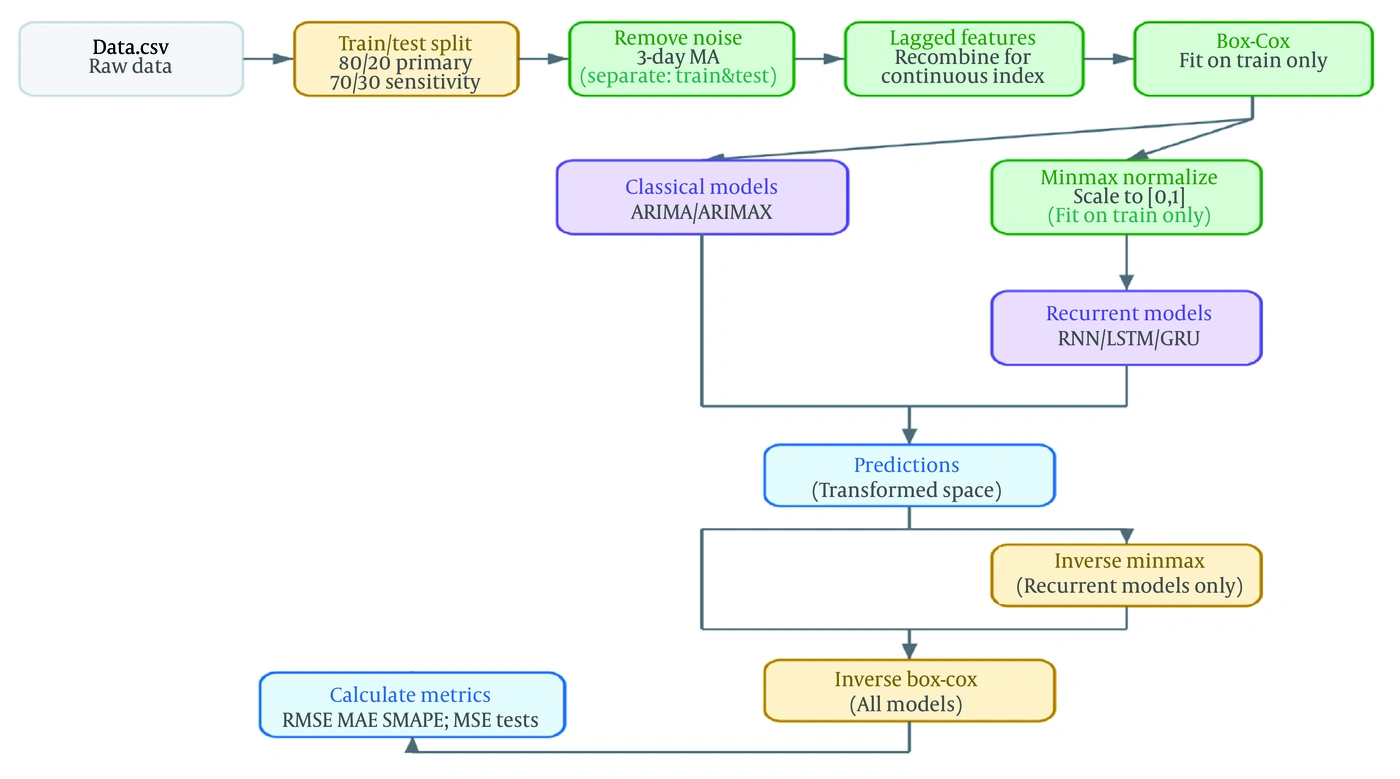
Figure 1.
Study workflow and leakage-control schematic
3.2. Preprocessing and Leakage Control
Records were ordered by date before modeling. Duplicate dates and missing daily values were assessed, and implausible values were verified against source records. The dataset contained no missing values for any variable across the full study period, as confirmed by the descriptive statistics in Table 2; therefore, no imputation or exclusion of observations was required. A causal trailing 3-day moving average was applied only to the environmental predictor series to reduce day-to-day measurement noise in the input variables. The mortality series was not smoothed; the forecast target was the raw observed daily cardiovascular death count for the following day.
where xt-1, xt-2, and xt-3 are the observed values on the three preceding days. Because this smoother relies exclusively on past observations, it contains no information from the current or future days, thereby maintaining leakage control.
Table 1.
CCF-Selected Lag Maps Across Model Families Within Each Train Fraction a
| Train fraction | CO | Humidity | NO2 | O3 | PM10 | SO2 | Temperature |
|---|---|---|---|---|---|---|---|
| 80% | 1 | 5 | 2 | 6 | 0 | 1 | 1 |
| 70% | 1 | 6 | 2 | 7 | 0 | 1 | 1 |
a Abbreviations: CCF, cross-correlation function; CO, carbon monoxide; NO2, nitrogen dioxide; O3, ozone; PM10, particulate matter with aerodynamic diameter less than 10 μm; SO2, sulfur dioxide.
The autocorrelation function (ACF) and partial autocorrelation function (PACF) were used descriptively to inspect temporal dependence in the mortality series and to inform the classical-model search without using held-out test observations.
Transformations that could use distributional information were fitted only on the training portion within each train fraction. The Box-Cox transformation was applied to reduce skewness and improve variance stability before model fitting (24). Min-Max scaling was subsequently used to place the input variables on a common numerical scale, facilitating stable optimization of the recurrent neural networks. Transformation and scaling parameters were estimated using only the development/training data and then applied to the corresponding held-out observations to prevent information leakage.
The fitted Box-Cox and Min-Max parameters were then applied unchanged to validation and test observations. Final forecast accuracy was calculated after reversing the fitted scaling and target transformation so that predictions and observed targets were compared on the raw daily mortality scale.
Cross-correlation screening for multivariate lag selection was performed using only the corresponding training portion. Candidate lags 0 to 7 were evaluated for each environmental predictor, and the lag with the largest absolute training-set cross-correlation was selected.
False discovery rate screening was recorded when the correlation passed the prespecified threshold. When no lag passed that threshold, the maximum-absolute-correlation lag was retained as a forecasting input, not as evidence of a statistically significant exposure lag. The held-out forecast period was not used for lag selection, transformation fitting, scaling, hyperparameter tuning, or early stopping.
3.3. Input Designs
Three input designs were evaluated. The univariate design used only past cardiovascular mortality and therefore included no environmental lag. The CCF-selected multivariate design incorporated environmental predictors at variable lags. For the CCF-selected multivariate design, candidate lags were evaluated using only the training portion. For each environmental predictor, the lag corresponding to the largest absolute cross-correlation with the mortality series within the prespecified candidate-lag range was selected. These lags represent the strongest empirical temporal associations observed in the training data within the evaluated lag range and were used solely to construct forecasting inputs. They were not interpreted as evidence of causal exposure-response relationships. The manual 7-day multivariate design incorporated all environmental predictors at lag 7.
The manual 7-day lag was selected based on a systematic preanalysis evaluation of candidate lags from 1 to 56 days, using RMSE on the training data as the selection criterion. Lag 7 emerged as the best-performing lag under this evaluation and was therefore retained as the manual multivariate input design. This selection was performed exclusively within the training portion to prevent information leakage from the held-out test period. Lag 7 should therefore be interpreted as an empirically selected forecasting design, not as evidence that all environmental predictors have a 7-day biological effect.
The CCF analysis identified consistent lag structures for the environmental and meteorological variables across the evaluated training fractions (Table 1). For the 80% training fraction, the selected lags were 1 day for CO, 5 days for humidity, 2 days for NO2, 6 days for O3, 0 days for PM10, 1 day for SO2, and 1 day for temperature. Using the 70% training fraction resulted in a highly similar lag structure, with only minor changes for humidity and O3 (6 and 7 days, respectively). Overall, the selected lags showed high consistency across training fractions, supporting the stability of the CCF-based lag-selection procedure.
3.4. Model Families
ARIMA was used as the univariate classical time-series baseline, and ARIMAX extended this baseline by adding lagged environmental predictors (25).
This distinction retained ARIMA as the mortality-history baseline and ARIMAX as the linear benchmark for the two multivariate input designs.
The neural comparison included a standard RNN, an LSTM, and a GRU (10-12). These models received fixed-length sequential inputs and produced one-step-ahead mortality forecasts using standard recurrent neural-network formulations. The study compared forecasting performance; it did not estimate causal exposure-response effects.
3.5. Model Training, Validation, and Hyperparameter Search
The primary evaluation used a fixed chronological 80/20 split. The earliest 80% of observations comprised the development period, and the most recent 20% comprised the held-out test period. A fixed chronological 70/30 split was used as a sensitivity evaluation. Within each development period, a terminal validation slice from the training portion supported hyperparameter selection and early stopping. The held-out test period was not used for order selection, transformation fitting, scaling, lag selection, hyperparameter tuning, or early stopping.
Classical ARIMA and ARIMAX models were fitted within each train fraction and input design using information-criterion-guided order selection. Candidate orders were searched within the training portion, and the selected order was the converged specification with the lowest prespecified information criterion among the converged models. Akaike information criterion (AIC) and Bayesian information criterion (BIC) values are reported as classical-model diagnostics, not as substitutes for held-out forecast accuracy.
Recurrent models were tuned separately for each model and input-design setting using a 40-trial random search conducted exclusively on the development data. The predefined search space included sequence length (7, 14, 28, 56, and 91 days), hidden dimension, dropout rate, learning rate, batch size, number of recurrent layers, training loss function, and early-stopping settings. Models were trained using mini-batch optimization for up to 200 epochs, with early stopping applied to the validation portion according to the prespecified patience criterion. The configuration achieving the best validation performance within the 40-trial search budget was selected for the final model. No test-set information was used during hyperparameter tuning or model selection; the test set was reserved exclusively for final out-of-sample evaluation.
All recurrent models were optimized using the Adam optimizer. Maximum training epochs were set to 200, with early stopping applied when validation loss did not improve for 15 consecutive epochs (patience = 15). Batch size was 16 for both train fractions. The five random seeds used across all evaluations were 11, 22, 33, 44, and 55. The validation slice comprised the terminal portion of the development data and was used exclusively for early stopping and hyperparameter selection.
All analyses were implemented in Python using the following packages: PyTorch (≥ 1.13) for recurrent models; statsmodels (≥ 0.13) for ARIMA, ARIMAX, and statistical tests; scikit-learn (≥ 1.1) for Min-Max scaling; scipy (≥ 1.8) for Box-Cox transformation; pandas (≥ 1.5) and numpy (≥ 1.22) for data handling; and PyWavelets (≥ 1.3) for wavelet decomposition.
The 70/30 split is an overlapping sensitivity analysis rather than an independent external validation; both splits draw from the same 10-year series and share a substantial training period. Its purpose was to assess whether primary RMSE rankings were sensitive to the choice of train fraction.
Each recurrent model setting was evaluated under five random seeds to quantify variation due to initialization, sampling, and optimization under the same fixed chronological split. Seeds were not treated as independent forecast observations. For each model and forecast date, seed-level losses were aggregated before final metric calculation and before MSE-based statistical comparison.
3.6. Accuracy Metrics and Statistical Comparison
Models were ranked descriptively by RMSE, with lower RMSE defining the best-ranked model within a comparison universe. Mean absolute error (MAE) and symmetric mean absolute percentage error (SMAPE) were reported as secondary metrics; SMAPE was used as the relative-error metric because it is symmetric in observed and predicted values and is unitless (26). Statistical comparisons used date-level MSE loss rather than aggregate RMSE values, preserving the forecast date as the independent comparison unit.
For transparency, SMAPE was calculated as:
where the summation is over the n held-out forecast dates, and yt and ŷt are the observed and predicted mortality values at forecast date t. Primary accuracy metrics were RMSE, MAE, and SMAPE, calculated over the held-out forecast dates.
For recurrent models with repeated seeds, seed-level date-specific losses were averaged before statistical comparison.
For each best-ranked model and competitor, paired date-level loss differences were used for winner-versus-competitor testing.
Model Confidence Set (MCS) analysis used date-level MSE loss with a moving-block bootstrap Tmax approximation, α = 0.05, and 1,000 bootstrap samples (27). Block length was 28 for both the 80/20 and 70/30 splits. MCS was used to assess whether the evaluated set could be reduced to one retained model or whether several models remained statistically close.
Winner-versus-competitor comparisons used Diebold-Mariano-style paired loss-difference tests on MSE loss, with Newey-West adjustment for autocorrelation in the loss-difference series and Holm correction within each comparison universe (28-30). These tests compared the best-ranked model with each competitor on the same forecast dates. The Newey-West adjustment was used because errors on adjacent forecast dates can be correlated, and the Holm correction was used because several pairwise comparisons were made within the same comparison universe.
Throughout the paper, a model is described as best-ranked when it has the lowest RMSE. A stronger claim of unique statistical superiority required support from both the MCS retained set and Holm-adjusted winner-versus-competitor tests.
The Friedman test was used as an omnibus sensitivity analysis of model loss ranks, not as a procedure for selecting a unique winner (31). A significant Friedman P value indicates that at least some model ranks differ in the comparison universe; it does not show which model is better than which competitor. Therefore, winner claims in this paper rely on RMSE ranking plus MCS and multiplicity-adjusted pairwise loss tests, not on the Friedman test alone.
Figure 2 summarizes the final evaluation path from the raw daily series to split-aware, seed-aware statistical comparison.
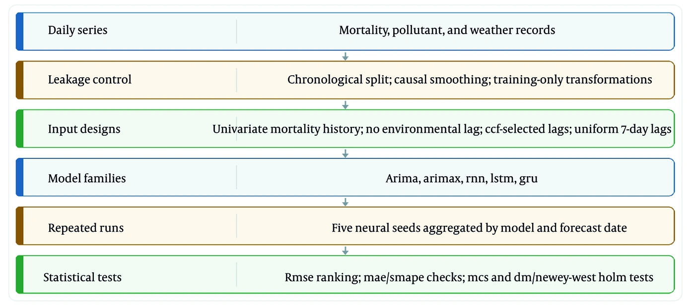
Figure 2.
Final evaluation process
3.7. Hyperparameter and Classical-Order Reporting
Neural hyperparameters were summarized across the five repeated-seed evaluations rather than from a single seed. Categorical settings are reported by mode, with tied modes stated when present; numeric settings are reported by median and interquartile range. No individual seed is highlighted as the preferred run. For ARIMA and ARIMAX, selected model order, AIC, and BIC are reported for each train fraction and input design in which the classical model was fitted. Information criteria describe in-sample classical-model fit and are reported separately from held-out forecast ranking.
4. Results
All performance metrics reported in this section—RMSE, MAE, and SMAPE—were calculated exclusively on the chronologically held-out test period. No training-set performance metrics are reported in the results tables.
4.1. Study Data and Evaluation Design
The dataset comprised 3,652 consecutive daily observations spanning approximately 10 years, providing a substantial continuous time series for model development, validation, and chronologically held-out evaluation. The primary 80/20 split provided 731 held-out forecast dates, while the 70/30 sensitivity split provided 1,096 held-out forecast dates. Given the time-series forecasting design, a conventional cross-sectional sample size or statistical power calculation was not considered appropriate; analytical feasibility was instead assessed based on the length and continuity of the available time series and the predefined chronological evaluation design.
Table 2 shows complete daily coverage for all variables across the 10-year study period. The mortality series was relatively stable, with a mean of about 15 deaths per day, whereas PM10 and nitrogen dioxide showed wider ranges, consistent with intermittent high-pollution days. Temperature covered cold and warm seasonal conditions, and relative humidity varied substantially in this arid urban setting. One impossible source humidity value above 100% was treated as a data-entry error for descriptive reporting; the reported descriptive maximum was 98.5%.
Table 2.
Descriptive Statistics of the Analysis Dataset a
| Variables | n | Mean | SD | Min | Q1 | Median | Q3 | Max | Missing |
|---|---|---|---|---|---|---|---|---|---|
| Daily cardiovascular deaths | 3652 | 15.40 | 1.41 | 11.00 | 15.00 | 15.00 | 16.00 | 25.00 | 0 |
| CO | 3652 | 2.29 | 1.01 | 0.00 | 2.00 | 2.00 | 3.00 | 10.00 | 0 |
| O3 | 3652 | 18.66 | 9.13 | 1.00 | 12.00 | 17.00 | 23.00 | 71.00 | 0 |
| NO2 | 3652 | 45.47 | 16.52 | 4.00 | 35.00 | 42.00 | 52.00 | 146.00 | 0 |
| SO2 | 3652 | 26.46 | 10.48 | 2.00 | 20.00 | 25.00 | 31.00 | 112.00 | 0 |
| PM10 | 3652 | 73.75 | 20.62 | 16.00 | 61.00 | 72.00 | 85.00 | 335.00 | 0 |
| Temperature | 3652 | 18.53 | 8.48 | -0.80 | 10.80 | 18.80 | 26.70 | 34.80 | 0 |
| Humidity | 3652 | 39.09 | 17.19 | 9.50 | 25.50 | 35.00 | 50.50 | 98.50 | 0 |
a Abbreviations: CO, carbon monoxide; NO2, nitrogen dioxide; O3, ozone; PM10, particulate matter with aerodynamic diameter less than 10 μm; Q1, first quartile; Q3, third quartile; SD, standard deviation; SO2, sulfur dioxide.
4.2. Primary Overall Ranking Under the 80/20 Split
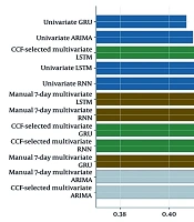
Table 3 shows that, under the primary 80/20 split, the univariate GRU was the best-ranked overall model by RMSE, with RMSE = 0.407, MAE = 0.322, and SMAPE = 2.061. The next closest model was the univariate ARIMA, with RMSE = 0.410, indicating that the classical univariate baseline remained a close comparator. The highest-ranked multivariate configuration was the CCF-selected multivariate LSTM (RMSE = 0.418) (Figure 3).
Table 3.
Primary 80/20 Overall Model Ranking a
| Rank | Model | Input design | RMSE | MAE | SMAPE | MCS retained |
|---|---|---|---|---|---|---|
| 1 | univariate GRU | Univariate | 0.407 | 0.322 | 2.061 | Yes |
| 2 | univariate ARIMA | Univariate | 0.410 | 0.327 | 2.100 | Yes |
| 3 | CCF-selected multivariate LSTM | CCF-selected multivariate | 0.418 | 0.331 | 2.127 | Yes |
| 4 | univariate LSTM | Univariate | 0.419 | 0.335 | 2.152 | Yes |
| 5 | univariate RNN | Univariate | 0.419 | 0.334 | 2.137 | Yes |
| 6 | manual 7-day multivariate LSTM | Manual 7-day multivariate | 0.430 | 0.343 | 2.203 | Yes |
| 7 | manual 7-day multivariate RNN | Manual 7-day multivariate | 0.432 | 0.344 | 2.205 | Yes |
| 8 | CCF-selected multivariate GRU | CCF-selected multivariate | 0.438 | 0.349 | 2.234 | Yes |
| 9 | CCF-selected multivariate RNN | CCF-selected multivariate | 0.442 | 0.353 | 2.268 | Yes |
| 10 | manual 7-day multivariate GRU | Manual 7-day multivariate | 0.444 | 0.355 | 2.279 | Yes |
| 11 | manual 7-day multivariate ARIMAX | Manual 7-day multivariate | 0.466 | 0.374 | 2.401 | No |
| 12 | CCF-selected multivariate ARIMAX | CCF-selected multivariate | 0.472 | 0.379 | 2.436 | No |
a Abbreviations: ARIMA, autoregressive integrated moving average; ARIMAX, ARIMA with exogenous variables; CCF, cross-correlation function; GRU, gated recurrent unit; LSTM, long short-term memory; MAE, mean absolute error; MCS, Model Confidence Set; RMSE, root mean square error; RNN, recurrent neural network; SMAPE, symmetric mean absolute percentage error.
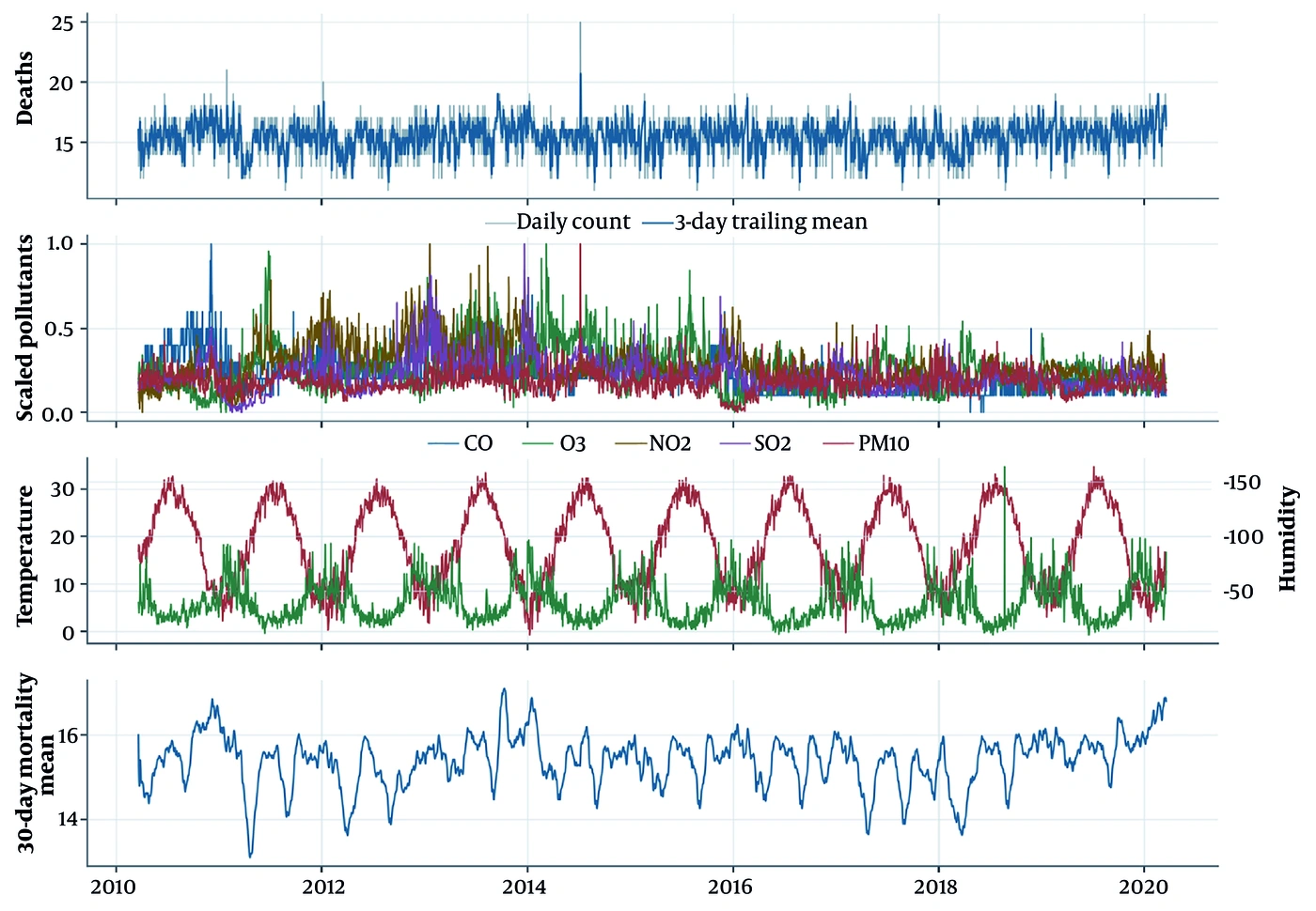
Figure 3.
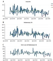
Study series over time
This ranking requires statistical qualification. The 80/20 overall MCS retained 10 of the 12 evaluated configurations, including the univariate GRU, the univariate ARIMA, and several recurrent univariate and multivariate alternatives. The univariate GRU was therefore best-ranked by RMSE, but the MCS did not support a unique statistical winner. Figure 4 visualizes this primary RMSE ranking and indicates which configurations remained in the retained MCS set. The absolute RMSE difference between the best-ranked univariate GRU, with RMSE = 0.407, and the univariate ARIMA, with RMSE = 0.410, was only 0.003. Relative to the mean daily cardiovascular mortality of approximately 15.4 deaths, this difference corresponds to roughly 0.02% of the outcome scale, indicating that the two models are practically indistinguishable on the primary metric.
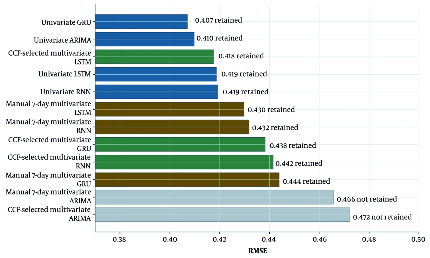
Figure 4.
Primary 80/20 overall root mean square error (RMSE) ranking
The most relevant best-performing configurations are those in the top rows of each overall comparison rather than a single isolated winner. Table 4 retains these top five configurations in the main text so that the reader can view the close alternatives, MCS-retained status, and Holm-adjusted winner-versus-competitor evidence alongside the descriptive RMSE ranking.
Table 4.
Top Five Best-Performing Overall Configurations Under Each Train Fraction a
| Train | Rank | Model | RMSE | MAE | SMAPE | MCS | Holm P | DM/Holm decision |
|---|---|---|---|---|---|---|---|---|
| 80% | 1 | univariate GRU | 0.407 | 0.322 | 2.061 | Yes | Reference | Best-ranked by RMSE |
| 80% | 2 | univariate ARIMA | 0.410 | 0.327 | 2.100 | Yes | 0.380 | Not significant |
| 80% | 3 | CCF-selected multivariate LSTM | 0.418 | 0.331 | 2.127 | Yes | 0.099 | Not significant |
| 80% | 4 | univariate LSTM | 0.419 | 0.335 | 2.152 | Yes | 0.099 | Not significant |
| 80% | 5 | univariate RNN | 0.419 | 0.334 | 2.137 | Yes | 0.058 | Not significant |
| 70% | 1 | univariate GRU | 0.399 | 0.308 | 2.014 | Yes | Reference | Best-ranked by RMSE |
| 70% | 2 | univariate ARIMA | 0.400 | 0.320 | 2.093 | Yes | 0.744 | Not significant |
| 70% | 3 | univariate RNN | 0.402 | 0.322 | 2.102 | Yes | 0.744 | Not significant |
| 70% | 4 | univariate LSTM | 0.407 | 0.305 | 1.996 | Yes | 0.303 | Not significant |
| 70% | 5 | manual 7-day multivariate GRU | 0.409 | 0.322 | 2.108 | Yes | 0.303 | Not significant |
a Abbreviations: CCF, cross-correlation function; DM, Diebold-Mariano; GRU, gated recurrent unit; LSTM, long short-term memory; MAE, mean absolute error; MCS, Model Confidence Set; RMSE, root mean square error; RNN, recurrent neural network; SMAPE, symmetric mean absolute percentage error.
Because the univariate GRU was the primary 80/20 RMSE winner, Figure 5 shows the observed and five-seed mean predicted mortality values for this model over the primary held-out test period. The plot shows the scale on which the primary errors were computed and helps interpret the small RMSE difference between the leading GRU and close alternatives.
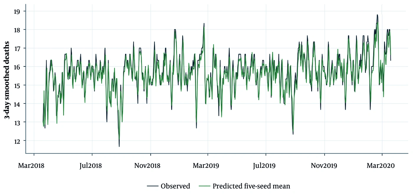
Figure 5.
Observed and predicted mortality in the primary test period
4.3. Performance by Input Design and Train Fraction
According to Table 5, the input-design results show why overall and within-design rankings should be interpreted separately. In the primary split, the univariate GRU led the univariate group, while the CCF-selected multivariate LSTM and manual 7-day multivariate LSTM led the two multivariate groups. In the 70/30 sensitivity split, the univariate GRU again led the univariate group, and GRU models led both multivariate groups. Multivariate winners therefore varied by training fraction and lag design, and the results do not support a stable overall gain beyond the best univariate baseline. Figure 6 summarizes this input-design sensitivity across the two training fractions.
Table 5.
Best-Ranked Models by Input Design and Train Fraction a
| Train Fraction | Input Design | Best-Ranked Model | RMSE | MAE | SMAPE | MCS Retained Summary | Friedman P Value |
|---|---|---|---|---|---|---|---|
| 80% | Univariate | univariate GRU | 0.407 | 0.322 | 2.061 | all 4 models retained | 6.052e-09 |
| 80% | CCF-selected multivariate | CCF-selected multivariate LSTM | 0.418 | 0.331 | 2.127 | 2 of 4 models retained: GRU, LSTM | 8.928e-07 |
| 80% | Manual 7-day multivariate | manual 7-day multivariate LSTM | 0.430 | 0.343 | 2.203 | 2 of 4 models retained: LSTM, RNN | 1.802e-08 |
| 70% | Univariate | univariate GRU | 0.399 | 0.308 | 2.014 | all 4 models retained | 4.268e-11 |
| 70% | CCF-selected multivariate | CCF-selected multivariate GRU | 0.413 | 0.320 | 2.093 | 3 of 4 models retained: GRU, LSTM, RNN | 0.154 |
| 70% | Manual 7-day multivariate | manual 7-day multivariate GRU | 0.409 | 0.322 | 2.108 | 3 of 4 models retained: GRU, LSTM, RNN | 0.168 |
a Friedman P values are omnibus tests on MSE loss with no multiple-comparison correction. Significant P values indicate that loss ranks differ somewhere within the comparison universe; they do not identify a unique best model. Abbreviations: CCF, cross-correlation function; GRU, gated recurrent unit; LSTM, long short-term memory; MAE, mean absolute error; MCS, Model Confidence Set; MSE, mean squared error; RMSE, root mean square error; RNN, recurrent neural network; SMAPE, symmetric mean absolute percentage error.
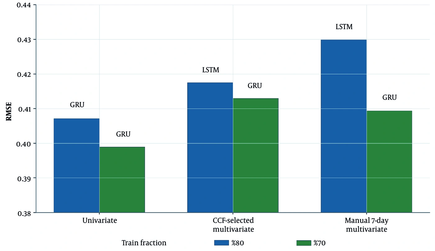
Figure 6.
Input design sensitivity across train fractions
4.4. Statistical Evidence for Close Competitors
Statistical comparisons support a cautious claim hierarchy. As summarized in Table 6, the 80/20 overall Friedman omnibus test on MSE loss was significant (P = 6.299e-34), and the 70/30 overall Friedman omnibus test was also significant (P = 9.082e-22). These tests indicate that loss ranks differ somewhere within the corresponding overall comparison universe, but they do not identify a single superior model. MCS results are therefore central to interpretation: in both training fractions, the overall MCS retained a broad set of close competitors rather than isolating the univariate GRU.
Table 6.
MCS and Friedman Statistical Summary a
| Train Fraction | Comparison Universe | Best-Ranked Model | MCS Retained Summary | Friedman P Value | Interpretation |
|---|---|---|---|---|---|
| 80% | All ARIMA, ARIMAX, RNN, LSTM, and GRU configurations | univariate GRU | 10 of 12 configurations retained | 6.299e-34 | Omnibus loss ranks differ; MCS does not isolate a unique winner |
| 80% | Univariate | univariate GRU | all 4 models retained | 6.052e-09 | Omnibus loss ranks differ; MCS does not isolate a unique winner |
| 80% | CCF-selected multivariate | CCF-selected multivariate LSTM | 2 of 4 models retained: GRU, LSTM | 8.928e-07 | Omnibus loss ranks differ; MCS does not isolate a unique winner |
| 80% | Manual 7-day multivariate | manual 7-day multivariate LSTM | 2 of 4 models retained: LSTM, RNN | 1.802e-08 | Omnibus loss ranks differ; MCS does not isolate a unique winner |
| 70% | All ARIMA, ARIMAX, RNN, LSTM, and GRU configurations | univariate GRU | 10 of 12 configurations retained | 9.082e-22 | Omnibus loss ranks differ; MCS does not isolate a unique winner |
| 70% | Univariate | univariate GRU | all 4 models retained | 4.268e-11 | Omnibus loss ranks differ; MCS does not isolate a unique winner |
| 70% | CCF-selected multivariate | CCF-selected multivariate GRU | 3 of 4 models retained: GRU, LSTM, RNN | 0.154 | Omnibus test is not significant; retained models remain statistically close |
| 70% | Manual 7-day multivariate | manual 7-day multivariate GRU | 3 of 4 models retained: GRU, LSTM, RNN | 0.168 | Omnibus test is not significant; retained models remain statistically close |
a MCS used date-level MSE loss with a moving-block bootstrap Tmax approximation, α = 0.05, and 1,000 bootstrap samples. The moving-block length was 28 forecast dates for both the 80/20 and 70/30 splits. Friedman P values are omnibus tests on MSE loss and were not adjusted for multiplicity. Abbreviations: ARIMA, autoregressive integrated moving average; ARIMAX, ARIMA with exogenous variables; CCF, cross-correlation function; GRU, gated recurrent unit; LSTM, long short-term memory; MCS, Model Confidence Set; MSE, mean squared error; RNN, recurrent neural network.
Winner-versus-competitor Diebold-Mariano (DM)/Newey-West tests with Holm correction were consistent with this qualified interpretation (Table 7). In the 80/20 overall comparison, the univariate GRU was significantly superior (Holm-adjusted) to both ARIMAX configurations and to the manual 7-day multivariate GRU, but was not significantly different from the univariate ARIMA, the CCF-selected multivariate LSTM, the univariate LSTM, or the univariate RNN. Thus, the descriptive RMSE ranking is not accompanied by statistical separation from the closest competitors. In the 70/30 overall comparison, three of the 11 MSE contrasts were significant after Holm correction: comparisons with CCF-selected multivariate ARIMAX, manual 7-day multivariate ARIMAX, and CCF-selected multivariate GRU. The overall DM/Newey-West Holm inventory contained 22 rows per split: 11 MSE contrasts used for inference and 11 MAE sensitivity contrasts.
Table 7.
Selected Overall DM/Newey-West Holm Contrasts for the Best-Ranked Model a
| Train Fraction | Winner | Comparator | Test and Loss | Holm P Value | Decision |
|---|---|---|---|---|---|
| 80% | univariate GRU | univariate ARIMA | DM/Newey-West on MSE | 0.380 | Not significant |
| 80% | univariate GRU | CCF-selected multivariate LSTM | DM/Newey-West on MSE | 0.099 | Not significant |
| 80% | univariate GRU | univariate RNN | DM/Newey-West on MSE | 0.058 | Not significant |
| 80% | univariate GRU | manual 7-day multivariate GRU | DM/Newey-West on MSE | 1.349e-09 | Significant |
| 70% | univariate GRU | univariate ARIMA | DM/Newey-West on MSE | 0.744 | Not significant |
| 70% | univariate GRU | CCF-selected multivariate GRU | DM/Newey-West on MSE | 0.042 | Significant |
| 70% | univariate GRU | manual 7-day multivariate GRU | DM/Newey-West on MSE | 0.303 | Not significant |
a Abbreviations: CCF, cross-correlation function; DM, Diebold-Mariano; GRU, gated recurrent unit; MSE, mean squared error.
Selected within-design pairwise comparisons reinforce the same point. In the 80/20 CCF-selected multivariate group, the CCF-selected multivariate LSTM was significantly separated from the CCF-selected multivariate GRU by DM/Newey-West testing on MSE loss with Holm correction (P = 0.016), although the MCS retained both models. In the 80/20 manual 7-day group, the manual 7-day multivariate LSTM was not significantly separated from the manual 7-day multivariate RNN (P = 0.304). In the 70/30 CCF-selected multivariate group, the CCF-selected multivariate GRU was not significantly separated from the CCF-selected multivariate LSTM (P = 0.435), and in the 70/30 manual 7-day group, the manual 7-day multivariate GRU was not significantly separated from the manual 7-day multivariate LSTM (P = 0.232).
4.5. Sensitivity Analysis Under the 70/30 Split
As an overlapping sensitivity analysis rather than an independent external validation, the 70/30 split assessed whether primary rankings were stable across training fractions. As shown in Table 8, the main overall RMSE ranking pattern was preserved. The univariate GRU remained the best-ranked overall model by RMSE, with RMSE = 0.399, MAE = 0.308, and SMAPE = 2.014. The univariate ARIMA was again a close second, with RMSE = 0.400, followed by the univariate RNN, with RMSE = 0.402, and the univariate LSTM, with RMSE = 0.407. Secondary metrics warrant caution: in the 70/30 split, the univariate LSTM achieved lower MAE (0.305 vs 0.308) and lower SMAPE (1.996 vs 2.014) than the univariate GRU, even though the GRU retained the lowest RMSE. This metric discordance underscores that the ranking of the leading models is sensitive to the choice of accuracy measure and that no single model dominated across all criteria.
Table 8.
70/30 Sensitivity Overall Model Ranking a
| Rank | Model | Input design | RMSE | MAE | SMAPE | MCS retained |
|---|---|---|---|---|---|---|
| 1 | univariate GRU | Univariate | 0.399 | 0.308 | 2.014 | Yes |
| 2 | univariate ARIMA | Univariate | 0.400 | 0.320 | 2.093 | Yes |
| 3 | univariate RNN | Univariate | 0.402 | 0.322 | 2.102 | Yes |
| 4 | univariate LSTM | Univariate | 0.407 | 0.305 | 1.996 | Yes |
| 5 | manual 7-day multivariate GRU | Manual 7-day multivariate | 0.409 | 0.322 | 2.108 | Yes |
| 6 | CCF-selected multivariate GRU | CCF-selected multivariate | 0.413 | 0.320 | 2.093 | Yes |
| 7 | CCF-selected multivariate LSTM | CCF-selected multivariate | 0.414 | 0.321 | 2.106 | Yes |
| 8 | manual 7-day multivariate LSTM | Manual 7-day multivariate | 0.415 | 0.321 | 2.101 | Yes |
| 9 | manual 7-day multivariate RNN | Manual 7-day multivariate | 0.417 | 0.334 | 2.182 | Yes |
| 10 | CCF-selected multivariate RNN | CCF-selected multivariate | 0.421 | 0.336 | 2.198 | Yes |
| 11 | manual 7-day multivariate ARIMAX | Manual 7-day multivariate | 0.457 | 0.368 | 2.405 | No |
| 12 | CCF-selected multivariate ARIMAX | CCF-selected multivariate | 0.460 | 0.370 | 2.416 | No |
a Abbreviations: ARIMA, autoregressive integrated moving average; ARIMAX, ARIMA with exogenous variables; CCF, cross-correlation function; GRU, gated recurrent unit; LSTM, long short-term memory; MAE, mean absolute error; MCS, Model Confidence Set; RMSE, root mean square error; RNN, recurrent neural network; SMAPE, symmetric mean absolute percentage error.
4.6. Model Settings and Classical Orders
Table 9 reports the key architecture and loss settings identified for the best-ranked neural models in the primary and sensitivity analyses. The optimal configurations varied across training fractions and input designs, although recurrent architectures remained among the leading models. In the 80/20 split, the overall and univariate rankings were led by the univariate GRU, using three recurrent layers, a sequence length of 14, and Huber loss. The CCF-selected and manual 7-day multivariate groups were led by LSTM models with two recurrent layers and L1 loss. In the 70/30 sensitivity split, the univariate GRU again ranked first overall and within the univariate group, while GRU models led both multivariate input designs. The corresponding CCF-selected lag maps are also reported in Table 1.
Table 9.
Essential Recurrent-Model Settings for Best-Ranked Neural Models a
| Train Fraction | Result Context | Model | Hidden Units | Layers | Sequence Length | Loss | Input |
|---|---|---|---|---|---|---|---|
| 80% | Overall and univariate | univariate GRU | 32/64 | 3 | 14 | huber | Mortality history |
| 80% | CCF-selected multivariate | CCF-selected multivariate LSTM | 32/32 (second tied with 64) | 2 | 56 (tie: 91) | l1 | CCF lag map |
| 80% | Manual 7-day multivariate | manual 7-day multivariate LSTM | 32/32 | 2 | 91 | l1 | All predictors at lag 7 |
| 70% | Overall and univariate | univariate GRU | 32/32 (first tied with 64; second tied with 64) | 3 | 56 | huber | Mortality history |
| 70% | CCF-selected multivariate | CCF-selected multivariate GRU | 16/32 (second tied with 64) | 2 | 14 | huber | CCF lag map |
| 70% | Manual 7-day multivariate | manual 7-day multivariate GRU | 32/16 (second tied with 32) | 3 | 56 | huber | All predictors at lag 7 |
a Abbreviations: CCF, cross-correlation function; GRU, gated recurrent unit; LSTM, long short-term memory.
For the classical models, Table 10 summarizes the selected ARIMA/ARIMAX orders and their corresponding information criteria. The univariate ARIMA models had lower AIC and BIC values than the corresponding multivariate ARIMAX models in both training fractions. In the 80/20 split, the univariate ARIMA had AIC = 16647.65 and BIC = 16695.48, compared with AIC values of 17317.09 and 17306.00 for the CCF-selected and manual 7-day ARIMAX models, respectively. A similar pattern was observed in the 70/30 split, where the univariate ARIMA had lower AIC and BIC than both multivariate ARIMAX configurations. These information-criterion results are consistent with the weaker descriptive performance of the multivariate ARIMAX models reported in the overall model rankings.
Table 10.
Classical Model Orders and Information Criteria a
| Train fraction | Model | Order | AIC | BIC |
|---|---|---|---|---|
| 80% | univariate ARIMA | [1,0,5] | 16647.6473045 | 16695.4847549 |
| 80% | CCF-selected multivariate ARIMAX | [5,1,0] | 17317.0909825 | 17394.7733231 |
| 80% | manual 7-day multivariate ARIMAX | [5,1,0] | 17306.0030759 | 17383.6809468 |
| 70% | univariate ARIMA | [5,0,3] | 15504.4516587 | 15562.9136469 |
| 70% | CCF-selected multivariate ARIMAX | [5,1,0] | 16034.8035667 | 16110.7378637 |
| 70% | manual 7-day multivariate ARIMAX | [5,1,0] | 16062.4464908 | 16138.3807877 |
a Abbreviations: AIC, Akaike information criterion; ARIMA, autoregressive integrated moving average; ARIMAX, ARIMA with exogenous variables; BIC, Bayesian information criterion; CCF, cross-correlation function.
5. Discussion
5.1. Principal Findings
Short-term cardiovascular mortality in Shiraz was predicted mainly from its own recent history. The univariate GRU had the lowest RMSE in both chronological splits. The absolute RMSE gaps were negligible relative to the scale of daily mortality (differences of 0.001 - 0.003 against a mean of ≈ 15.4 deaths). Combined with the MCS retaining 10 of the 12 evaluated configurations in both splits, these results indicate that the choice among the leading models is less consequential than maintaining a robust, leakage-controlled forecasting pipeline. The results identify a small set of usable forecasting candidates, with the GRU as the most consistently leading model.
This pattern is plausible for daily city-level mortality data. Cardiovascular deaths are temporally structured, but they are also aggregate outcomes shaped by reporting routines, population age structure, access to care, seasonality, and recent health conditions. A recurrent model can learn part of this short-term structure, whereas the close performance of ARIMA indicates that classical baselines retain practical value.
Many of these structural factors (reporting routines, population age structure, healthcare access, and recent health conditions) are already reflected, at least indirectly, in the recent mortality series itself. This may explain why strong univariate models based solely on mortality history performed so competitively.
5.2. Environmental and Epidemiological Interpretation
Air pollution and weather remain important cardiovascular concerns. The narrower question here was whether CO, O3, NO2, SO2, PM10, temperature, and humidity improved short-term mortality forecasts beyond the information already contained in recent mortality. Under the tested input designs, they did not provide a stable overall gain.
One plausible explanation for this limited forecasting contribution is that city-level daily averages cannot capture fine-scale spatial and temporal exposures—such as neighborhood gradients, indoor and occupational environments, heat stress, and acute dust episodes—that may trigger cardiovascular events in susceptible individuals. As a result, these aggregated measures often add little independent predictive information beyond what is already reflected in recent mortality history.
This finding should not be interpreted as evidence that environmental exposures are unimportant for cardiovascular disease. Epidemiological relevance and forecasting value are different standards. Environmental variables improve prediction only when they are measured at an appropriate spatial and temporal scale, lagged correctly, and provide information that is not already contained in the recent mortality series.
5.3. Model Interpretation and Public-Health Use
The multivariate results also temper expectations about adding predictors or using more flexible models. ARIMAX did not lead the multivariate comparisons, and the best recurrent multivariate model differed between train fractions. Additional inputs can add signal, but they can also introduce noise, instability, or lag mismatch. For this dataset, a strong mortality-history baseline was the more reliable starting point.
For public health practice, these models are best viewed as surveillance tools rather than causal explanations. A forecasting system based on the univariate GRU—or, given their statistical indistinguishability, the classical ARIMA baseline—could support several operational functions: 1) daily surveillance dashboards that flag predicted mortality increases to public health teams, enabling early activation of response protocols; 2) short-term hospital capacity planning, including bed allocation and staffing adjustments during predicted high-mortality periods; 3) integration with air-pollution and heat-warning systems to provide composite risk signals during pollution episodes or extreme temperature events; and 4) population-level monitoring in other arid Iranian cities with similar mortality and environmental profiles, pending prospective validation. Before operational deployment, the model should be recalibrated periodically with incoming data, validated prospectively, and benchmarked against simple persistence baselines to confirm that predictions remain reliable under changing conditions.
5.4. Strengths, Limitations, and Future Work
This study has several strengths, including the analysis of a decade of daily cardiovascular mortality and environmental records from a large arid city, direct comparison of classical and recurrent models, the use of separate univariate and multivariate input designs, implementation of repeated neural-network seeds, and the application of split-aware statistical testing.
Regarding model performance, the lack of significant improvement when incorporating environmental variables suggests that city-level daily averages may fail to capture the fine-scale exposures that trigger cardiovascular events. Instead, factors such as reporting routines and population structure appear to be captured indirectly by mortality history, which likely accounts for the strong performance of univariate models. Furthermore, we did not assess whether the modest advantage of the univariate GRU was consistent across the entire test period or concentrated in specific subperiods; therefore, date-level error trajectories remain an open question for future work.
The evaluation was further limited by the absence of rolling-origin resampling, naïve persistence and seasonal-naïve benchmarks, and uncertainty intervals for the principal performance metrics. The moving-block bootstrap block length was selected based on calendar considerations rather than a formal data-driven procedure. These represent important directions for future work.
The current study focused on forecast accuracy comparison rather than model interpretability. Future work could apply permutation-based variable importance or SHapley Additive exPlanations (SHAP)-based attribution to the multivariate recurrent models to identify which environmental predictors contribute most to forecast accuracy, with the caveat that such metrics reflect predictive contribution under a specific model architecture rather than causal or epidemiological importance.
Our analysis is limited to a historical period ending in March 2020. Given that the COVID-19 pandemic substantially altered cardiovascular mortality patterns, health care utilization, and reporting practices, prospective validation with post-2020 data is essential before any operational deployment of these models. Future research should test the proposed pipeline prospectively, evaluate other Iranian cities, and examine age- and sex-specific CVD mortality if data access permits. Finally, investigating richer environmental indicators—such as heat, dust, pollution episodes, and exposure summaries over multiple lags—may clarify the conditions under which environmental inputs enhance forecasts versus when recent mortality history alone suffices.
5.5. Conclusions
Daily cardiovascular mortality forecasting in Shiraz was driven most consistently by recent mortality history. The univariate GRU was the best-ranked model by RMSE in both the 80/20 primary split and the 70/30 sensitivity split, but it was not uniquely superior; ARIMA and several recurrent models remained statistically close.
Environmental variables are epidemiologically important for CVD, but in this forecasting exercise they did not consistently improve prediction beyond the strongest univariate baseline. The findings support a cautious surveillance strategy: start with a robust mortality-history model, test environmental extensions prospectively, and update the system with newer data, subgroup analyses, and richer exposure measures before routine early-warning use.