

1. Background
By measuring oxygen extraction fraction (OEF) in the brain tissue in all conditions of rest and functional activity, important information of brain functionality in both health and disease could be achieved (1). In addition, the human brain is at most about 2% of the whole body weight, but it nearly consumes 20% of the body’s oxygen supply (2).
Developing a reliable technique for whole brain oxygen mapping could lead to a better understanding of normal physiology in any condition which could also be of great help in situations with disturbance in oxygen supply. Previous studies have shown that hypoxia (lack of oxygen in tissue) in tumors could affect the response to therapies, metastasis, aggressiveness and local recurrence and thus aggravate the overall prognosis (3).
To calculate oxygen consumption, several parameters have been introduced. The most important ones are cerebral metabolic rate of oxygen consumption (CMRO2) and oxygen extraction fraction (OEF). OEF could be defined as the fraction of oxygen that is removed from the blood flowing through by the brain tissue (1, 2). It is extremely uniform in baseline condition (resting state which is the awake state with eyes closed).
As the brain uses most of the energy budget in the baseline condition and activity represents only a small increasing change, understanding its functionality could lead to understanding of the normal performance of the human which is essential for baseline abnormality due to diseases such as stroke and Alzheimer. For instance, in patients with cerebrovascular diseases, OEF has been an accurate predictor in later strokes (4). Also, other brain disorders, such as Parkinson, Alzheimer and Huntington disease, and multisystem atrophy, contain changes in cerebral oxygen metabolism (3).
To have an acceptable oxygen mapping method, some standards should be considered, such as sufficient temporal and spatial resolution, noninvasiveness, quantification of oxygen level, no radiation exposure, high safety and availability in all clinics. Currently none of the in vivo methods contains all of these requirements (3).
The gold standard for OEF imaging is positron emission tomography (PET) that involves a sequence of three scans with injection of 15O or 18F that is about 46 min and meanwhile the patient is exposed to a radiation dose of 8300MBq (5).
PET imaging has several disadvantages that limit its use. It is not widely available and it requires radioactive isotope at the start of the cyclotron which is why it is not repeatable in the same subject. It also has low resolution, long imaging time, and it is expensive.
The development of blood oxygen level dependent (BOLD) MRI by Ogawa et al. created a new tendency in the noninvasive study of brain hemodynamic. BOLD imaging is based on the fact that deoxygenated and oxygenated bloods have different magnetic susceptibilities and the magnetic susceptibility of the deoxygenated blood is similar to that of the tissue. In theoretical models of BOLD contrast, BOLD signal is related to hemodynamic parameters such as deoxyhemoglobin concentration, deoxyhemoglobin containing blood volume (DBV), CMRO2 and OEF (1).
In comparison with PET imaging, MR imaging is safe, noninvasive, widely available in clinics, repeatable and cheap. Also with a proper method, all images could be acquired within a short time and it could be done with all standard MRI scanners.
After the development of BOLD imaging in 1990, several methods have been proposed for OEF measurements in whole brain or a single vein which could give some valuable information in normal cases but in the presence of neuronal abnormality or tumors, it can not provide local information. Methods such as An and Lin (2000) (6), Lu and Zijl (2005) (7), Lu and Ge (2008) (8), Huppert (2009) (9), Xu (2009) (10), Jain (2010) (11) and Qin (2011) (12) could be placed in this category and TRUST and VASO methods are the most known of them.
Some other methods for OEF measurements need primary assumption of cerebral blood volume (CBV) and tried to show the OEF as a map in a limited part of the brain. Studies conducted by Domsch and Mie (2001) (13), He and Yablonskiy (2007, 2008) (1, 4), and Bolar (2011) (14) are based on such procedures.
The latest methods that have been developed for OEF measurement are based on a combination of hyperoxic and hypercapnic stimulus while acquiring ASL data. Gauthier and Hoge (2012) (15) and Bulte (2012) (5) where the first group that used these methods. In the following years (2013, 2016), wise et al. (16, 17) made some improvement to these methods and gained more accurate results for OEF.
2. Objectives
As ASL is a new imaging technique and is limited in some scanners, we proposed a new method for OEF measurement based on calibrated BOLD model which uses dynamic susceptibility contrast (DSC) perfusion imaging instead of arterial spin labelling (ASL) with two injections of contrast agent in hyperoxic and baseline state and BOLD imaging while applying hperoxic and hypercapnic stimulus.
 image")
The paradigm of gas manipulation while acquiring blood oxygen level dependent (BOLD) image
| Parameters | WM | GM | Whole Brain |
|---|---|---|---|
| CBF0 | 769.9022 ± 55 | 2541.329 ± 201 | 1761.1 |
| M | 3.5329 ± 0.32 | 5.2017 ± 0.47 | 4.044 |
| [dHb] / [dHb]0 | 0.8819 ± 0.003 | 0.9107 ± 0.004 | 0.9053 |
| OEF | 0.3719 ± 0.022 | 0.4601 ± 0.016 | 0.4403 |
Mean Value of Estimated Parameters in GM, WM and Whole Braina
3. Materials and Methods
3.1. Imaging
This project was approved by Islamic Azad University (south branch), and the data acquisition was done at Imam Khomeini hospital, NIAG (Neuro imaging and analysis group), with a 3T Siemens Trio Tim scanner, a transfer body coil and an 8 channel receiver head coil. Five subjects (three males, two females) were recruited for this study with at least five different regions of interest (ROI) of each to calculate the mean value in gray matter (GM), and white matter (WM). The subjects were selected from the patients with a low- grade tumor on one side of their brain.
The BOLD data was acquired with an echo planar imaging (EPI) sequence while performing the changes in gas inhalation within 13 minutes in 40 slices of the brain with: 260 volumes, repetition time (TR) = 3000 ms, echo time (TE) = 30 ms, Slice Thickness = 3, Flip angle = 90° and resolution = 64 × 64.
The DSC perfusion data, one with normal breathing and the second one with hyperoxic stimulus, was acquired with an EPI sequence, 40 slices, 80 volumes, TR = 2230 ms, TE = 30 ms, Slice Thickness = 3, Flip angle = 70°, resolution = 64 × 64.
Also a T1 structural image was acquired with: 176 slices, TR = 1800 ms, TE = 3.44 ms, TI = 1100 ms, Slice Thickness = 1, Flip angle = 7° and resolution = 256 × 256.
3.2. Gas Manipulation
The 13 minutes of BOLD imaging consists of manipulating the inhalation gas, which is a combination of normoxia, hypercapnia, and hyperoxia. The paradigm for gas manipulation is shown in Figure 1.
 in a single subject. As expected, gray matter (GM) has higher values than white matter (WM) and the brain shape is complete and clear. The tumor has a low OEF because of the inactive tumor, which is necrosis and is completely clear in the map.")
Slice 3 to 40 for oxygen extraction fraction (OEF) in a single subject. As expected, gray matter (GM) has higher values than white matter (WM) and the brain shape is complete and clear. The tumor has a low OEF because of the inactive tumor, which is necrosis and is completely clear in the map.
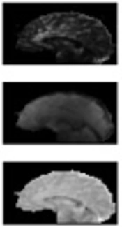
![Cerebral blood flow (CBF0), M, [dHb]/[dHb]<sub>0</sub>, and oxygen extraction fraction (OEF) respectively in slice 20 in one of the subjects](https://services.brieflands.com/cdn/serve/3170b/5a17fb916885c84ab6bd46539aea098035257171/iranjradiol-In_Press-In_Press-64253-i003-preview-preview.webp "Cerebral blood flow (CBF0), M, [dHb]/[dHb]<sub>0</sub>, and oxygen extraction fraction (OEF) respectively in slice 20 in one of the subjects")
Cerebral blood flow (CBF0), M, [dHb]/[dHb]0, and oxygen extraction fraction (OEF) respectively in slice 20 in one of the subjects
| Paper | Year | Short Description of the Method | CBF0 (mL/100 g/s) | OEF |
|---|---|---|---|---|
| Lu and Zijl (7) | 2005 | Multi-Echo VASO GE-fMRI | - | 0.23 |
| He abd Yablonskiy (4) | 2007 | qBOLD | - | 0.38 |
| Lu ang Ge (8) | 2008 | TRUST | - | 0.352 |
| Jain et al. (11) | 2010 | SVO2 in the superior sagittal sinus with MR susceptometry-based oximetry | 2664 | 0.35 |
| Domsch and Mie (13) | 2014 | Nimp qBOLD | - | 0.46 |
| Bolar et al. (14) | 2011 | QUIXOTIC | 3360 | 0.26 |
| Gauthier and Hoge (15) | 2012 | Combination of GCM and hypercapnic and hyperoxic stimulus using ASL | 2600 | 0.35 |
| Bulte et al. (5) | 2012 | Combination of calibrated BOLD with hypercapnic and hyperoxic stimulus using ASL | 2460 | 0.38 |
| Wise et al. (16) | 2013 | Combination of calibrated BOLD with hypercapnic and hyperoxic stimulus using ASL(modified) | 3330 | 0.4 |
| Our Study | 2016 | Combination of calibrated BOLD with hypercapnic and hyperoxic stimulus using DSC-Perfusion & BOLD | 2541 | 0.46 |
Comparison of Mean Values of OEF and CBF0 in Different Methods
The inspired gases were delivered via a single tube connected to a nasal cannula. At normoxic condition, no gas was delivered and the subject breathed the environment air. At hypercapnia, a capsule was connected to the tube with a gas combination of 8% CO2, 21% O2 and 71% N2, which by using a nasal cannula, it was combined with the environmental air and 4% CO2 was applied. The hyperoxic condition was the same, and the gas capsule that was used consisted of 79% O2 and 21% N2 to provide 50% of O2 for the subjects. The capsules were changed manually in normoxic conditions and the gas delivery was set to 10 L/min.
Moreover, the measurement of the OEF at rest was based on the differences in cerebral blood flow (CBF) (please refer to the appendix). The CO2 level in hypercapnia was considered with the probability of gaining a stronger CBF, with the condition that it would not harm the subject. The O2 level in hyperoxia, was the most suitable level so that the blood flow would not decrease because of the increase in blood oxygen. This level of hypercapnia and hyperoxia creates a proper condition for OEF calculation.
3.3. Analysis
Smoothing and motion correction was done as the preprocessing step with SPM12 (MATLAB). The CBF estimation was done using ASIST (PMA) software, and the results were used with the BOLD data to estimate OEF by MATLAB coding.
The coefficients α and β were set at 0.2 and 1.3, using previous studies as reference (5).
PaO and PaO2 (end-tidal partial pressure of oxygen at rest and hyperoxia respectively) can be measured using Capnograph. Here the mean values of previous studies (18) were used for PaO and PaO2 in all subjects, and were set at 110 and 300, respectively.
4. Results
Table 1 contains the average values of CBF0, M, [dHb] / [dHb]0 and OEF at GM, WM and whole brain with the standard deviation for the measurements in GM and WM ROIs.
Note that the normal side of the brain is considered in all measurements so it could be compared to the normal values of other studies. The ROIs for normal parts were mainly selected in the normal contra lateral hemisphere of the same patient. The ROIs for WM were mostly selected from the periventricular region, and in the GM, from the frontal cortex.
The OEF map of one of the subjects is shown in Figure 2 and the brain image, with different values of OEF in different regions (higher values in GM and lower values in WM) is completely obvious. In addition, considering a low value of CBF in the tumor part, which is known as necrosis, as expected has a lower value of OEF as well. As OEF scale is in fraction, it does not have any unit and its range is between 0 and 1. In Figure 3, the map of different parameters that was calculated during the OEF analysis is shown for a single slice in a sample subject. The baseline CBF is shown with the unit of mL/100 g/s. Moreover, as M and [dHb] ratio is proportional to fractions, they do not have a unit.
5. Discussion
Here we proposed a new method for calculating OEF based on calibrated BOLD model with hypercapnia and hyperoxia stimulus and two times injection of contrast agent for DSC perfusion, one in normoxic and one in hyperoxic condition. The normal range for OEF at rest is between 0.3 and 0.5 (19). The mean value of OEF for GM and WM has been calculated as 0.46 and 0.37, respectively (Table 1), which is within the standard range and is considered as acceptable.
As expected, GM has a higher value than WM and all the maps show a clear vision of the brain structure. Even the low grade tumor shows a low value of OEF because it has low perfusion.
PET imaging is the gold standard for OEF measurement and mapping. The normal OEF estimated value in PET imaging has been reported as 0.44 by Ito et al. in 2004) (20).
Mean normal value of GM in several MRI methods has been shown in Table 2. Previous studies in OEF measurement with MRI all share the same purpose, to have the most accurate OEF value in any ROI with an appropriate mapping that could be applied in all MRI scanners. The results of several studies have been shown in Table 2. These results are comparable with the values of the proposed method.
Each method has its own advantage and disadvantages. The proposed method could be considered the most available one as it only uses EPI and BOLD imaging sequences and no additional hardware is needed (just two capsules). This method is more likely similar to those of previous studies that use hypercapnia and hyperoxia stimulus except that instead of ASL imaging, the combination of BOLD and DSC-perfusion has been used and the expected three times injection of contrast agent for OEF calculation at rest has been decreased to only two injections.
Having an accurate value for OEF leads to appropriate diagnosis of diseases such as stroke, Alzheimer, Parkinson, and Huntington (3, 4, 15), as well as better prediction which helps to reach effective precautions.
The proposed method here has the advantage of having a simple structure that could be done with any MRI scanner that has the ability to acquire EPI data and even the switching between gases could be done manually. By considering these factors, this method could be considered as the most available one in all clinical scanners.
In conclusion, the presented method uses the combination of hyperoxia and hypercapnia stimulus with BOLD calibration model and DSC perfusion imaging for CBF calculation, that could be applied in any MRI scanner and could be considered as the most available one in all clinical and research scanners.
The voxel wise estimation allows any ROI calculation of the parameters especially OEF and the data acquired have enough information to estimate other important parameters such as CBV, initial area under the curve (IAUC), cerebrovascular reverse (CVR) and CMRO2. The calculated values are absolute and are comparable to those from PET imaging studies yet with no radiation and with lower cost.
