


1. Background
Nowadays, computed tomography (CT) is critical for the technical aspects of three dimensional (3D) conformal radiotherapy and image-guided external radiation therapy dose planning. CT images provide a relationship between tissue electron density and voxel values to set up accurate dose calculations, which depend on the attenuation properties of the tissue and generation of digitally reconstructed radiographs (DRRs) (1). In recent years, interest has been developing in replacing CT scan images with MRI images in the treatment planning process. This is due to the fact that MRI provides a high soft tissue contrast that could improve the determination of target tissue and the accuracy of risk volume delineation in organ at risk (OR). The advantages of planning directly on MRI scans include numbers of functional imaging options, no ionizing radiation for the patient, and reduction in costs (1-4).
Higher contrast in the soft tissue can lead to better separation of tumor tissue from the organ at risk and determine the exact size of the tumor area (5). Furthermore, MRI can be used before, during, and after treatment for patient follow-up without being concerned about patients receiving ionizing radiation (6). MRI is going to be used as a tool for image-guided radiotherapy (IGRT), where MRI-Cobalt and MRI-Linac are being developed and even these machines have been used in some limited radiation therapy centers (7). In the treatment planning dose calculation in MR-Linac, the entire patient volume is assumed as water equivalent electron density. Furthermore, assuming a homogeneous density compared with planning heterogeneously can lead to dose discrepancies greater than 2%. So, the tissues in the MR image were classified into different classes such as soft tissue and bone (and in some cases air) by manual contouring from T1-weighted MR images and every class was assigned an electron density (8).
Nowadays, based on fusion of MRI images with CT scan slices in soft tissue structures, both images can be taken advantage of simultaneously (9). Nevertheless, in addition to increased extra costs and scan time using multiple modalities, fusion techniques have limitations (10). In MRI-only based systems in which the CT modality is eliminated completely, in addition to solving the extra cost, time and limitation issues, brain segmentation could be performed more accurately and more comfortably (11).
Alongside all these advantages, geometric distortions due to non-uniformities of the magnetic field, gradient nonlinearity, and patient-induced susceptibility are some limitations that must be properly investigated in an MRI-only radiation planning to produce accurate treatment planning and dose calculation. (12-14). Also, a significant problem in MRI-alone radiation planning systems, however, is that scans cannot be calibrated to electron density value due to different imaging protocols. There are different methods to provide an electron density map, one of which is rigid registration of MRI images on CT images. Unfortunately, this method will be so difficult when the patient’s position is slightly different between MRI and CT imaging (2, 14, 15). Several researchers have investigated the possibility of removing CT modality from radiation therapy planning and implementing an MR-only simulation system (16-19). Different methods have been developed to estimate the electron density information from MRI for external radiation therapy in recent years. Bulk density assignment involves applying an area of interest within the MRI to single homogeneous density values for manual contouring. The main benefit of the method is its manageability, though the calculation results may not be as accurate as CT for constructing reliable DRRs (14, 15, 20-24). Atlas-based registration methods involve registering target MRI to a single CT to generate a substitute CT, which can be a simple approach, unlike accurately mapping complex anatomy. Atlas-based approaches are currently the only fully automated methods for generating pseudo-CT images by converting a single standard MRI sequence to CT, and are more robust to intensity differences between images. The main disadvantage is that the registration algorithms used may be unable to deform atlas images to match anatomical properties which are missing from an atlas-training set (25).
A semi-automated segmentation has been proposed through a deformable registration of a selected atlas (26). A conjugated electron-density mapping atlas and whole MRI atlas based on the manually delineated MRI scans have been generated by Dowling et al. (16). An optimization approach based on the robust block-matching has been proposed which utilizes a half-way space definition to maintain inverse-consistency (27). Also, a half space transform and its inverse have been optimized simultaneously by a robust symmetric registration algorithm (28). Synthesizing CTs from MR images has been done using an iterative multi-atlas approach due to morphological similarity of the mapped atlases to the target (29). To learn the intensity mapping with atlas-based approaches, most regression methods rely on a training set of co-registered CT-MR scans. Other studies have investigated the use of Gaussian Mixture Regression and Random Forest Regression for creating a pseudo-CT image from dual ultra-short echo time (dUTE) and m-Dixon MRI images (30, 31). In addition to the two methods mentioned, another way in creating pseudo-CT images is voxel-based methods that are embedded in two groups based on the use of functional MRI sequences: the standard sequences and the ultrashort echo time sequences (UTE). In the study (32), pseudo-CTs were generated using a voxel-based, weighted summation method using ultrashort echo time phase images from a weighted combination of water fat maps and unwrapped UTE phase maps. CT image HUs values and T1/T2 weighted MRI intensity values were utilized to generate a model conversion technique from MR intensity by applying a second-order polynomial model (33). In (34), a voxel-wise tissue classification was applied to derive pseudo-CT for optimization ion radiotherapy treatment plans. Pseudo-CT was created with an inversely modulated radiotherapy (IMRT) plan based on an assigning electron density to an anatomic image (35). The purpose of the study (36-38) is to establish pseudo-CT generation using an undersampled ultrashort echo time (UTE)-mDixon pulse sequence by a linear combination of the fuzzy c-means (FCM) membership functions. In the studies (38-40), substitute CT images were derived by Gaussian mixture regression.
2. Objectives
The CT scan, despite numerous benefits, does not reveal accurate information about the soft tissue contrast, which is often difficult to distinguish the target tissues of the organ at risk and to determine the volume of the tumor in a typical RT programming. Also, the main challenge is that the brain MRI cannot map the bone very well. The bone signal is lost before being read because of the short T2 value, and there is no direct correlation between the intensity of the resonance imaging and electron density. CT images include such information, as the intensity in these images is directly related to the electron density of the tissue and provides an accurate geometry of the bone. The main goal of this study was to investigate the possibility of removing the CT simulator from the therapeutic process and replacing it with pseudo-CT images and calculating the electron density values for designing patient treatment planning. It is investigated whether there is a relationship between MRI intensity and CT-HU value within different brain regions. The purpose is to find a simple and efficient model that could provide electron density information from the MRI images to generate the synthetics-CT images with an acceptable error rate that could be used in clinical RT treatment planning. Segmentation of the bones was performed by the Fuzzy C-means algorithm in these images.
3. Materials and Methods
The MRI was performed by a 1.5 T SIEMENS medical scanner. Repetition time (TR) was 400 ms, Echo time (TE) was 10ms, flip angle was 90, Bandwidth (BW) was 90.9 kHz, and matrix size was 512 × 512. The brain CT images were taken by a SIEMENS scanner, at 120 kVp with the slice thickness of 2mm, and 512 × 512 in-plane image dimensions.
Ten randomly chosen patients were prescribed external brain RT (five men and five women, age 20 to 71 years, mean age of 45 years). The patient’s agreements were obtained after they were informed about the whole procedure of the study.
This project did not have any effect on the treatment planning of these patients. Eight patients were included in the generation of the model, while two others were considered for independent validation. At first, the series of CT images and MRI images were segmented by the FCM clustering algorithm including soft tissue (brain), air and bone. Clustering is an unsupervised learning algorithm whereby the samples are divided into categories whose members are similar to each other that are called clusters. The cluster is, therefore, a set of objects that are similar to each other and are identical to objects in other clusters. Indeed, agents were selected for input samples and then based on their similarity with the samples, the selected cluster could be determined, which was repeated until the agents of clusters did not change (41). For each patient 10, 25 and 5 voxels were chosen randomly within the skull bone, brain, and sinus area, respectively. The corresponding MRI intensity values and CT values of different voxels in different areas created the data points for the generation and validation of the models. The skull voxels were chosen uniformly within the segmented bone volume.
The purpose was to assess the overall relationship between MRI intensity and CT-values in different segmented parts of the brain with sufficient accuracy for radiation therapy planning. The electron density values should be determined from the MRI intensity values. We considered the air regions in CT and MRI series as similar. The model fit is illustrated in Figure 1 for the brain and skull region.
 number of voxels within the brain and skull bones")
The relationship between MRI intensity and Hounsfield unit (HU) number of voxels within the brain and skull bones
We can use simple polynomial models (1st and 2nd order) for these parts.
Brain: A = 0.01563, B = 1042
Skull: A = -0.9004, B = 2381
Brain: A = 3.955 ×10⁻⁶, B = 0.013, C = 1043
Skull: A = 0.003709, B = -1.915, C = 2429
Where, MRintensity and A, B, C represent the MR intensity value and fitting parameters of the regression model, respectively. The parameters include complex functions of the tissue component fractions as well as T1 and T2 value within a voxel of MR image. The order for the polynomial fit was chosen based on the mean absolute error between pseudo-CT and simulated CT. Figure 2 displays the whole process of the algorithm by a simple flowchart.

The whole process flowchart
4. Results
We chose two simple models for different segmented parts of the brain and bone area to be applied on the test MR images. Figure 3 reveals the simple result of the process.

An example of segmentation of images with the aim of creating pseudo-CT using regression models
As the figure indicates, the head area is segmented into different regions by the FCM algorithm. Considering the interrelationships between the data extracted from the image series, and applying them on the test MR values to form pseudo-CT images, the desired result could be achieved.
Figure 4 presents the results of applying the 1st polynomial model to different slices of the head. Two simple models for different segmented parts of the brain and skull region were selected for application to the test MR images.

Pseudo-CT generation using regression models for three different slices of the head
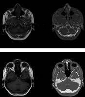
Two models were applied to test the segmented images in order to demonstrate model functionality. The difference between the three segments in the original and pseudo-CT image can be observed in Figure 5.

Images in the first row show the original MRI and CT slices. The 2nd and 3rd rows show the pseudo-CT images generated by the 1st-order polynomial model along with their differences between the original and pseudo-CT in the brain, skull, and air region. The 4th and 5th row represent the pseudo-CT images which are generated by the 2nd-order polynomial model along with their differences between original and pseudo-CT in the brain, skull, and air region respectively.
For further investigation, Figure 6 reveals the histogram chart of the differences between a selected region in the head and skull region of a pseudo-CT image and the original CT scan using the two models presented in the previous section.

Images in the first column represent the original CT slices. Images in the second column show the pseudo-CT images generated by the two models, and images in the third and fourth columns indicate the differential histograms between the original and pseudo-CT images in the brain and skull region, respectively.
The pseudo-CT images could be compared with the original CT images to verify their characteristics. Possibly, the simplest and the most common measurement scale is the measure of voxel-wise mean absolute error and the mean error as below:
Where, N is the total number of MR voxels in the different segments, where the CT and pseudo-CT are arranged in a vector of 1 * N. They contain the intensity values of the CT and the pseudo-CT in the same location. Table 1 provides the results of the mean absolute error and the mean error for different sections of the head, by applying the polynomial models with the 1st and the 2nd order.
| Error | Brain: 1st order; skull: 1st order | Sub-image 1st model | Brain: 2nd order; skull: 2nd order | Sub-image 2nd model | ||||||
|---|---|---|---|---|---|---|---|---|---|---|
| Brain | Skull | Air | Brain | Skull | Brain | Skull | Air | Brain | Skull | |
| Upper slice | ||||||||||
| ME | 0.7479 | 0.334 | -0.0433 | 7.0088 | -40.944 | 0.7477 | 0.34 | -0.0433 | 11.523 | 10.266 |
| MAE | 23.55 | 33.999 | 2.395 | 19.6195 | 116.528 | 23.60 | 33.91 | 2.395 | 14.498 | 117.051 |
| Middle slice | ||||||||||
| ME | -0.53 | -0.082 | 0.0145 | 16.759 | -61.276 | -0.53 | -0.060 | 0.0145 | 16.20 | -60.335 |
| MAE | 19.40 | 50.53 | 1.226 | 18.5366 | 119.635 | 19.43 | 50.41 | 1.226 | 18.118 | 119.780 |
MAE and ME Results for Polynomial Models in the Sub-Image Part
5. Discussion
A relationship has been indicated between the intensity of MR image and CT-based planning (relative electron density information) within the different brain regions with this type of MRI protocol. There is no need for special protocol and multiple MR series to replace CT. The regression relationships between MRI intensity and the relative electron density value from synthetic CT were obtained via the first- and 2nd-order polynomial regression models. An advantage of the proposed method is better distinction of tumor tissue from normal tissue in pseudo-CT images rather than typical CT scan images. It is due to the differences in tumor and normal tissue intensity in MR image and this difference could also be observed after mapping in pseudo-CT image. So the exact tumor delineation can be performed in pseudo-CT as well as MR image. The provided conversion models were validated inside different regions of the head in an independent patient group by choosing the voxels randomly and manually. The results suggested that the 2nd-order model did not generate less error than the first-order model. Because the amount of errors were too close and it could be concluded that by making models more complex, we cannot necessarily expect better results. The correlation values, resulting from the pseudo-CT images and measured CT scans of the patient that were being tested were 0.9682, 0.6389, and 0.7296 in different areas of the brain, skull, air, and sinuses, respectively. It is found that this level of correlation is appropriate in the brain region. The parameter value for the structural similarity index (SSIM) in these images was also equal to 0.8080, 0.9823, and 0.8921, respectively.
The SSIM can be used for measuring image quality by pseudo-CT image and original CT images as the reference image. In the following, the correlation and SSIM value between the whole complete pseudo-CT image and measured images were 0.8567, and 0.6023, respectively. In this article, there were less error rates than similar methods in voxel-based articles. In a study conducted by Kapanen and Tenhunen, results are obtained on the pelvic bone area and the MAE of the conversion model was 135 HU, while in this article, distinct models have been created on different brain regions with the use of FCM and contouring segmentation (23). The presented model creates appropriate images in terms of graphical observations of the structure of the skull bones and mean square errors. According to the imaging protocol (T1/T2*-weighted), in Kapanen and Tenhunen’s study, the results were sensitive to bone segmentation errors (23). Nonetheless, in this study, with the help of convenient segmentation techniques, separation of the skull bone from the air region was appropriate and we were able to separate these areas fairly well and create pseudo-CT images with presented regression models. Andreasan et al. used a Gaussian mixture regression (GMR) model with k-means clustering and an EM algorithm to train the model and generate the pseudo-CT by dUTE protocol and add the mDixon images. Nonetheless, these images are not a common protocol in MRI imaging and can limit clinical applications. In addition, the value of the mean absolute prediction error was carried out as 148HU in their study (42). Other methods such as patch-based regression model and multi-atlas approach based on affine registrations were implemented by Anderson, and 87, and 97 HU mean absolute error (MAE) errors were gained (30, 43). The results show that the errors obtained in this study reached the desired level. As a future work, the clinical uncertainty which is related to computing the electron density value by presented conversion models could be clinically tested and become more acceptable.
