


1. Background
With the increasing prevalence of kidney stones each year, the need for urgent treatment of this condition and its associated complications is strongly felt. It is estimated that 900,000 people develop kidney stones in the United States (1). Prevention and treatment of patients with kidney stones mainly depend on the type of kidney stone and its composition (2). The treatment of kidney stones may involve adequate hydration and urine alkalization (3), endoscopic methods, dietary modifications, or antibiotic prescriptions, depending on the stone type (4).
Computed tomography (CT) scan has been accepted as an accurate modality for the diagnosis of abdominal diseases (5, 6). Non-contrast CT scan of the abdomen and pelvic regions is considered the standard method for diagnosis of ureterolithiasis, with high sensitivity and specificity (7). Abdominal/pelvic single-energy CT scans provide information on the size, location, and attenuation values of urinary stones (8). However, dual-energy CT (DECT) scan has been proposed for the in vivo analysis of the chemical composition of kidney stones. This technique can differentiate between uric acid and non-uric acid stones (9). Commonly, the biochemical analysis of kidney stones is performed when the stones are removed from the body; therefore, an accurate in vivo composition analysis may prove effective for the treatment planning of patients.
Generally, DECT plays a significant role in identifying the chemical composition of kidney stones in vivo and therefore, selecting a more effective therapeutic plan (medical and/or surgical). Despite these advantages, DECT has some limitations, including hardware complexity, high cost, low accessibility, and most importantly, high radiation dose to patients (10). Several studies have shown that the DECT technique increases the received patient dose (11). Therefore, it seems necessary to develop an accurate and rapid technique using ultra-low-dose (ULD) CT or single-energy CT (SECT) for patient dose reduction.
In recent years, neural networks, also known as deep learning (DL) algorithms, have gained considerable attention in classification, segmentation, and image generation tasks (12-16). Several studies have focused on automated methods based on DL for identifying the urinary stone composition ex vivo. Serrat et al. indicated the role of kidney stone classification in reducing the recurrence rate (17). They proposed an automated method by evaluating 454 kidney stones and feature extraction. Overall, 80% of the samples were classified in the correct class, and an overall accuracy of 63% was achieved (17, 18).
Moreover, Black et al. assessed the application of DL method to automatically identify 63 different compositions of human kidney stones based on digital images, using the pre-trained ResNet-101 convolutional neural network (18). Additionally, Martinez et al. proposed an effective supervised learning method to increase the accuracy of kidney stone classification using a ureteroscopic analysis (19). Lopez et al. also conducted a study on kidney stone identification based on endoscopic images using a deep neural network (20). They compared five classification methods focusing on deep convolutional neural networks (DCNNs), with 98% and 97% precision and recall, respectively (20).
2. Objectives
In this study, we aimed to specify the kidney stone composition on SECT or ULD CT scans using deep neural networks. We proposed a DL-based classification method, focusing on the use of CT images. Human kidney stones were placed on an anthropomorphic phantom, and several ULD CT and DECT images (a pair of SECTs) were acquired to collect the input data. Human kidney stones were categorized based on DECT and biochemical reports. Deep neural networks were used to determine the stone type based on SECT or ULD CT scans.
3. Patients and Methods
3.1. Stone Preparation
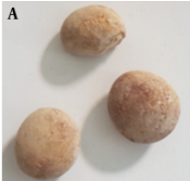
Several kidney stone samples were collected from 80 males and 66 females after removal by surgical procedures. The mean age of the patients was 42.5 ± 16.3 years (range, 16 - 69 years). After obtaining approval from the Institutional Research Ethics Committee, informed consent was obtained from all individuals, whose samples were used in this study. All the stones were sent to the chemical laboratory for further analysis after being washed with deionized water to remove debris. The samples were analyzed using the manual method of Darman Faraz Kave Company kit in Motahari Clinic Laboratory, Shiraz, Iran. The stone types were first determined via biochemical analysis in the pathology laboratory and then by DECT scans (Section 2.2). Stone samples with similar laboratory and DECT results were used in this study. A total of 146 pure samples of three different stone types were finally selected (Figure 1).

Three groups of kidney stones: A, Uric acid; B, Calcium oxalate; and C, Cystine
The three kidney stone types can be described as follows:
(1) Uric acid (C5H4N4O3) stones (5 - 10% of all kidney stones) are more common in men and formed by uric acid oversaturation in acidic urine (53 samples);
(2) Calcium stones (80% of all kidney stones) are the most common type of kidney stones. They can be found in two types: Calcium oxalate (CaC2O4.H2O-CaC2O4.2H2O) and calcium phosphate (Ca10(PO4)6(OH2)) (55 samples);
(3) Cystine stones ((-SCH2CHNH2COOH)2) (< 1% of all kidney stones) are a rare type of kidney stones that are formed when there is a high amount of cystine in the urine (38 samples).
3.2. CT Imaging Protocols
The kidney stones of known compositions were inserted in the kidney position of an Alderson Rando phantom, which is molded of tissue-equivalent materials and designed for imaging and dosimetry research (21, 22) (Figure 2). In the next step, spiral scanning was performed by a single-source DECT scanner (Aquilion Prime One, Toshiba, Japan).

A, Phantom preparation; and B, Phantom imaging
For identification of the kidney stone type using a DECT scanner, first, a large field-of-view ULD CT scan of the abdomen was acquired to determine the location of renal stones. Subsequently, DECT scan with a small field of view was acquired from the kidney stone area. It should be noted that DECT is not used for the entire abdomen and does not expose patients to high doses. Therefore, two scans were performed for each stone sample. In the first scan, to determine the stone position in the phantom, ULD CT scans (dose < 1.9 mSv) were acquired based on the SECT protocol, using a 3D adaptive iterative dose reconstruction (AIDR) technique with dose reduction features (23). The scanning parameters were as follows: 120 kVp; 15 mA; gantry rotation time, 0.5 sec; detector width, 0.4 mm; slice interval, 0.5 mm; slice thickness, 5 mm; and dose-length product (DLP), 4.90 mGy.cm.
The second scan was performed via single-source DECT with rapid voltage switching technique switching, focusing on the stone region. The acquisition parameters were as follows: 135 kVp and 15 mAs; 80 kVp and 92 mAs; and DLP, 48.40 mGy.cm. As can be seen, the DLP of 135-kVp CT imaging was 10 times higher than that of ULD CT at 120 kVp.
3.3. Stone Classification Based on DL Frameworks
In this step, four pre-trained 2D CNN classification networks were selected and trained in multiple training settings, based on the Taguchi parametric optimization method. The prepossessed stone images were inserted into four different deep networks, i.e., ResNet-50, ResNet-18, GoogLeNet, and VGG-19. Next, the classification efficiency of the four networks was compared. The results of biochemical analysis in the pathology laboratory and DECT predictions were used as the gold standard in this study. Pre-trained networks, which were trained in a large dataset (ImageNet), showed reasonable responses in previous research on classification tasks (24) The networks were customized, and the last two layers were tuned to update the net weights. Finally, optimization parameters, obtained from the Taguchi method, were set for the best of four pre-trained 2D CNN models to classify the stones into three different groups. The stages of the study are summarized in Figure 3.

A schematic view of the study steps
3.3.1. Taguchi Method
The Taguchi method is a simple statistical approach, consisting of multiple factors and levels to determine and classify the optimized parameters. It uses orthogonal array (OA) tables for the optimization process in the experimental design (25, 26). In this study, the Taguchi method was used to achieve optimal training combinations of hyperparameters for the networks. Six effective factors and three levels were considered on the training part of the networks (Table 1). To reduce the number of experiments, 27 experimental tests generated by Minitab-19 were conducted for the pre-trained ResNet-50, ResNet-18, GoogLeNet, and VGG-19 networks (Table 2).
| Factors | Level 1 | Level 2 | Level 3 |
|---|---|---|---|
| Solver | SGDM | ADAM | RMSPROP |
| Initial learning rate | 0.001 | 0.0001 | 0.0005 |
| Mini-batch | 32 | 64 | 128 |
| L2 regularization | 0 | 0.05 | 0.0001 |
| Drop factor | 0 | 0.1 | 0.95 |
| Drop period | 10 | 30 | 50 |
Levels of Solvers and Hyperparameters Designed by the Taguchi Method
| Experiment number | Factors | |||||
|---|---|---|---|---|---|---|
| A | B | C | D | E | F | |
| Solver | Initial learning rate | Mini-batch | L2 regularization | Drop factor | Drop period | |
| 1 | SGDM | 0.001 | 32 | 0 | 0 | 10 |
| 2 | SGDM | 0.001 | 32 | 0 | 0.1 | 30 |
| 3 | SGDM | 0.001 | 32 | 0 | 0.95 | 50 |
| 4 | SGDM | 0.0001 | 64 | 0.05 | 0 | 10 |
| 5 | SGDM | 0.0001 | 64 | 0.05 | 0.1 | 30 |
| 6 | SGDM | 0.0001 | 64 | 0.05 | 0.95 | 50 |
| 7 | SGDM | 0.0005 | 128 | 0.0001 | 0 | 10 |
| 8 | SGDM | 0.0005 | 128 | 0.0001 | 0.1 | 30 |
| 9 | SGDM | 0.0005 | 128 | 0.0001 | 0.95 | 50 |
| 10 | ADAM | 0.001 | 64 | 0.0001 | 0 | 30 |
| 11 | ADAM | 0.001 | 64 | 0.0001 | 0.1 | 50 |
| 12 | ADAM | 0.001 | 64 | 0.0001 | 0.95 | 10 |
| 13 | ADAM | 0.0001 | 128 | 0 | 0 | 30 |
| 14 | ADAM | 0.0001 | 128 | 0 | 0.1 | 50 |
| 15 | ADAM | 0.0001 | 128 | 0 | 0.95 | 10 |
| 16 | ADAM | 0.0005 | 32 | 0.05 | 0 | 30 |
| 17 | ADAM | 0.0005 | 32 | 0.05 | 0.1 | 50 |
| 18 | ADAM | 0.0005 | 32 | 0.05 | 0.95 | 10 |
| 19 | RMSPROP | 0.001 | 128 | 0.05 | 0 | 50 |
| 20 | RMSPROP | 0.001 | 128 | 0.05 | 0.1 | 10 |
| 21 | RMSPROP | 0.001 | 128 | 0.05 | 0.95 | 30 |
| 22 | RMSPROP | 0.0001 | 32 | 0.0001 | 0 | 50 |
| 23 | RMSPROP | 0.0001 | 32 | 0.0001 | 0.1 | 10 |
| 24 | RMSPROP | 0.0001 | 32 | 0.0001 | 0.95 | 30 |
| 25 | RMSPROP | 0.0005 | 64 | 0 | 0 | 50 |
| 26 | RMSPROP | 0.0005 | 64 | 0 | 0.1 | 10 |
| 27 | RMSPROP | 0.0005 | 64 | 0 | 0.95 | 30 |
The Taguchi L27 Orthogonal Array Parameter Setting in the Experiments
Based on the Taguchi optimization technique, the signal-to-noise ratio (SNR) was selected as the optimization criterion according to Equation 1, and the “larger-is-better” performance characteristics were preferred. The average SNR for each factor was calculated for 27 experiments, and the optimal levels of parameters were selected based on the highest SNR (25, 27):
where n is the total number of replications per test run, and yi is the accuracy of 2D CNN in the replication experiment.
3.3.2. Data Preparation and Pre-processing of CT Images
The CT images with a matrix size of 512 × 512 were collected at three energy levels (80 and 135 kVp for DECT scan and 120 kVp for ULD CT scan). To acquire raw CT data, each time, a stone was placed in an empty hole, in the kidney region of a Rando phantom, and the remaining space was filled with water. The Digital Imaging and Communications in Medicine (DICOM) slices were selected from volume CT phantom images of the stones and saved as 2D slices because of using 2D convolutional networks. The slices were then converted to PNG format. Due to the small size of the stones, some pre-processing procedures were applied to the images.
The images were cropped using the nearest neighbor method, and extra margins were removed with binary masks. The pixel intensities of the stone region were transferred to masked images via multiplication, and the normalization intensity was in the range of 0 - 255. Since the image size in all pre-trained networks was 224 × 224 × 3 pixels, all images obtained at each of the three CT energy levels were first resized accordingly before entering the networks. Bicubic interpolation was used to increase the resolution of images before feeding them into the networks. The images were then sorted into three categories based on the stone type. A total of 2200 slices from 146 CT scans were collected and categorized to prepare the final dataset. Figure 4 shows the dual CT images and stone locations, followed by the Hounsfield unit (HU) graph at 80 and 135 kV, indicating the type of stones. Processing was performed using the CT scan software. The preprocessing procedure for image preparation is also described.

A, Phantom images acquired by 80-kV X-ray; B, 135-kV X-ray; C, Stone type determination using the scanner software algorithm; D, Stone region; and E, Preprocessing for creating the stone dataset in deep networks
3.3.3. Network Architecture
The four pre-trained networks were run based on the training setup, described in Table 2, in the DL toolbox environment of MATLAB 2021. The training and validation accuracy and losses of networks were analyzed, and the results were inserted in Minitab software to select the optimized parameters. The dataset was divided into three sets (1600 images for training, 400 images for validation, and 150 images for tests) to avoid overlaps. The training and validation datasets were then augmented (random reflection axis [x, y]; random rotation, 0° - 20°; and random rescaling, 0.1 - 1) to improve the accuracy of the models. All experiments were run for 10 epochs to obtain high training and validation accuracies. Owing to the constant trends of training and validation procedures after six epochs, 10 epochs appeared to be sufficient. Each experiment was repeated five times to confirm the repeatability of the results of the training process. The dropout layers in each network helped prevent overfitting in the training procedure. The ResNet CNN architecture (Figure 5) yielded higher training and validation accuracies, besides fewer losses.

The ResNet CNN architecture
3.4. Performance Evaluation and Statistical Analysis
This study was conducted using the Deep Learning Toolbox of MATLAB 2021a on a system with the following setup: operating system, Windows 10 (enterprise/home); CPU, Intel® Core™ i7-10700 (3.5 GHz); GPU, NVIDIA GeForce RTX 3080; and RAM, 32 GB. According to the test procedure and estimation of the network performance, the confusion matrix was estimated. Generally, a confusion matrix is a table used to evaluate the performance of a classification network. The sensitivity (i.e., true positive rate), positive predictive value (ratio of true positive results to all positive results), negative predictive value (ratio of true negative results to all negative results), specificity (probability of a negative test result in subjects without disease), F-score, and accuracy were calculated based on the confusion matrix (Equations 2 - 5).
where TP is the number of true positives, TN is the number of true negatives, FP is the number of false positive results, and FN is the number of false negative results. The receiver operator characteristic (ROC) curves were drawn for different energy levels to evaluate the performance of the networks. Generally, the ROCs plot sensitivity versus 1-specificityon the X axis. This curve is used for the evaluation of classifiers and shows the trade-off between sensitivity and specificity. The further the curve comes to the 45° diagonal of the X-Y coordinate, the more accurate the network is.
To compare the performance of different networks, it would be helpful to summarize and show the performance of a predictive model with a single value. This single value can be the area under the ROC curve (AUC), which corresponds to the Wilcoxon rank-sum statistic. This value is used as a general measure of predictive accuracy (28). In other words, the ROC curve is a probability curve, and the AUC represents the measure or degree of separability. The AUC of the ROC curve is usually calculated to determine and compare the performance of predictive models. The AUC indicates how much the model can distinguish between different classes. The higher the AUC of the ROC curve is, the better the model performs in classification. Finally, one-way analysis of variance (ANOVA) was used for analyzing the results of stone type classification for different X-ray energies.
4. Results
4.1. DL Results
The prepared datasets were inserted in four different networks, and the training and validation accuracies were surveyed for different hyperparameters (Table 3). The results of the trained networks were evaluated, and training and validation accuracies and losses were compared. The GoogLeNet and VGG-19 networks were overfitted; their maximum training and validation accuracies did not exceed 70% and 60%, respectively. The best results with the highest accuracy and lowest loss values were attributed to the ResNet-18 and ResNet-50 networks for each energy. Table 3 shows the best results for ResNet-18 and ResNet-50 networks among 27 training sets. As shown in Table 3, the ResNet-50 exhibited better results at 80 kVp, while at 120 and 135 energies, ResNet-18 showed higher accuracy.
| Energies and trained network parameters | ResNet-18 | Experiment number | ResNet-50 | Experiment number |
|---|---|---|---|---|
| 80 kV | 16 | 27 | ||
| Training accuracy | 93 | 94.7 | ||
| Validation accuracy | 92.7 | 94.6 | ||
| Training loss | 0.8 | 0.1 | ||
| Validation loss | 0.2 | 0.19 | ||
| 120 kV | 15 | 27 | ||
| Training accuracy | 96 | 87 | ||
| Validation accuracy | 88.7 | 89.52 | ||
| Training loss | 0.1 | 0.33 | ||
| Validation loss | 0.5 | 0.4 | ||
| 135 kV | 26 | 26 | ||
| Training accuracy | 93.75 | 84 | ||
| Validation accuracy | 84.12 | 76 | ||
| Training loss | 0.27 | 0.4 | ||
| Validation loss | 0.36 | 0.6 |
The Best Results of ResNet-18 and ResNet-50 Networks Based on Hyperparameters Proposed in Taguchi Experiments
The most important factor in the Taguchi optimization method is SNR, which was calculated based on the Taguchi method (Figure 6). The effective parameters in the network performance were scored from one to six, based on the SNR (Table 4). According to the Taguchi method, the optimized arrangement of training options to achieve acceptable results was obtained.
 values of Taguchi method at different energy levels")
The signal-to-noise ratio (SNR) values of Taguchi method at different energy levels
| Parameters | 80 kV ResNet-50 | 120 kV ResNet-18 | 135 kV ResNet-18 |
|---|---|---|---|
| Solver | 6 | 2 | 1 |
| Initial learning rate | 2 | 6 | 5 |
| Mini-batch size | 1 | 3 | 4 |
| L2 regularization | 3 | 4 | 2 |
| Drop factor | 5 | 5 | 6 |
| Drop period | 4 | 1 | 3 |
Scoring of Effective Parameters at Each Energy Level Based on Taguchi Method a
4.2. Deep Neural Network Performance and Statistical Analysis
Figure 7 presents the results of confusion matrix and the ROC curve for the optimized parameters at each energy level in the performance evaluation of networks. Networks with high accuracy and low loss values were tested with the test dataset. The confusion matrix, F-score, and sensitivity were determined for the selected networks. The test accuracies were measured to be 92.7%, 89.5%, and 88.9% for 80, 120, and 135 kV energy levels, respectively. The AUCs for the three stone classes, i.e., uric acid, calcium oxalate, and cystine stones, at each energy level were estimated at 0.994, 0.997, and 0.940 at 80 kV; 0.938, 0.978, and 0.867 at 120 kV; and 0.958, 0.957, and 0.869 at 135 kV, respectively, all of which were close to one; therefore, the classifier networks used in this study were successful in stone type classification.
 curves for A, 80 kVp; B, 120 kVp; and C, 135 kVp energy levels (class 1: uric acid stones, class 2: cystine stones, class 3: calcium oxalate stones)")
Confusion matrices and receiver operator characteristic (ROC) curves for A, 80 kVp; B, 120 kVp; and C, 135 kVp energy levels (class 1: uric acid stones, class 2: cystine stones, class 3: calcium oxalate stones)
Table 5 indicates the mean values of parameters, along with 95% confidence intervals (CIs) for the networks. Based on the results of one-way ANOVA, there was a significant difference in the mean values of accuracy and sensitivity of classification for the three energy levels. The P-values for accuracy and sensitivity were 0.00002 and 0.003, respectively. No significant difference was observed regarding other scoring parameters (P > 0.05). The 80-kVp energy tests showed higher accuracy and sensitivity than the other two energy levels. However, there was no significant difference in the mean scores at 80, 120, and 135 kVp energy levels. Based on the results shown in Table 5, high evaluation scores for the three energy levels show the high performance of deep neural networks in stone composition identification at all three energy levels.
| Energy | F1-score mean (95% CI) | Sensitivity mean (95% CI) | Specificity mean (95% CI) | Positive predictive value Mean (95% CI) | Negative predictive value Mean (95% CI) | Accuracy mean (95% CI) |
|---|---|---|---|---|---|---|
| 80 kV | 0.84 (0.8, 0.89) | 0.8 (0.75, 0.85) | 0.95 (0.92, 0.99) | 0.94 (0.91, 0.96) | 0.96 (0.95, 0.97) | 0.90 (0.88, 0.92) |
| 120 kV | 0.75 (0.68, 0.81) | 0.67 (0.62, 0.71) | 0.90 (0.85, 0.95) | 0.86 (0.75, 0.96) | 0.94 (0.93, 0.95) | 0.84 (0.81, 0.88) |
| 135 kV | 0.85 (0.81, 0.89) | 0.70 (0.66, 0.73) | 0.90 (0.86, 0.94) | 0.89 (0.85, 0.93) | 0.92 (0.88, 0.97) | 0.84 (0.82, 0.92) |
The Evaluation Scores for Each Energy Level
The results indicated that the deep networks could predict the stone types based on the ULD CT images. Although the networks showed the highest accuracy and sensitivity at 80 kVp, ULD CT scan was preferred at a higher energy level (120 kVp) and a lower tube current (44 mA) with regard to the dose delivered to patients. Finally, the results of biochemical laboratory tests, network prediction, and DECT scanner output for determination of stone type were compared for six of the test samples (Table 6). The findings of the proposed method were matched with the pathology reports as the reference and confirmed the classification accuracy.
| Number of samples | Chemical analysis as the gold standard response | DECT Scan Results | ResNet-50 predictions at 80 kV |
|---|---|---|---|
| Sample 1 | UA stone | UA stone | 100% UA |
| Sample 2 | UA stone | UA stone | 99.9% UA |
| Sample 3 | CaOx stone | CaOx stone | 99.1% CaOx |
| Sample 4 | CaOx stone | CaOx stone | 93.3% CaOx |
| Sample 5 | Cys stone | Cys stone | 99.6% Cys |
| Sample 6 | Cys stone | Cys stone | 98.1% Cys |
Comparison of Pathology Test, CT Scan Output, and Network Prediction Results
5. Discussion
Kidney stones, if left untreated, can lead to kidney pyelonephritis or renal failure in more serious cases; consequently, they may significantly affect the patient’s quality of life and also impose a major financial burden on the healthcare system. Prevention and treatment of patients with kidney stones mainly depend on the type of kidney stone and its composition (29). Cystine stones, despite being rare, are associated with genetic defects causing cystinuria; consequently, treatment typically involves adequate hydration and urine alkalization (3). Endoscopic methods are usually selected for cystine stone management, while uric acid stones may be prevented and treated by dietary modifications. In contrast, struvite stones are often associated with urinary tract infections, which require antibiotic treatments (4); therefore, stone type determination is very important.
There are various common methods for the ex vivo analysis of kidney stones (30). The DECT method with two different energy spectra can be used for in vivo characterization of the chemical composition of renal stones larger than 3 mm in size. Determination of the chemical structure of stones helps physicians treat them more effectively and facilitates the selection of treatment planning strategies (pharmaceutical treatment vs. surgery). However, DECT has some limitations, including increased patient radiation dose and the need for post-processing software systems of stone analysis (31).
In this study, a classification method with high accuracy was proposed using a DL approach. The dataset was collected using surgically collected human kidney stones, which were analyzed using chemical procedures. The imaging procedure was performed using DECT and SECT modalities on a pseudo-human phantom. Four pre-trained networks were selected according to acceptable responses in medical experiments, and the Taguchi optimization method was designed. Among four networks, two networks, including GoogLeNet and VGG-19, were excluded from our study owing to their poor performance in 27 Taguchi tests. However, ResNet-50 and ResNet-18 were used for optimization and training of parameters based on their high accuracy and low error rate. Overall, GoogLeNet has fewer trainable parameters than ResNet-50 and ResNet-18; therefore, it plays an effective role in training. On the other hand, the performance of ResNet networks does not decrease despite deepening of the architecture compared to other architectural models. Also, computations become lighter, and the network training ability is improved.
The ResNet-50 and ResNet-18 were trained using 27 proposed tests of Taguchi method for each of the three energies. For 80 kVp, the highest training and validation accuracies of the ResNet-50 network were 94.7% and 94.6%, respectively, while at 120 and 135 kVp, the ResNet-18 network showed better performance. The training and validation accuracies of ResNet-18 at 120 kVp were 96% and 88.7%, respectively; the corresponding values were 93.75% and 84.12% for ResNet-18 at 135 kVp, respectively.
Data analysis indicated interesting results. The highest mean factor and SNR were obtained for the 15th, 26th, and 27th experiment numbers of the Taguchi analysis (Table 5). The ranked hyperparameters of various energies indicated that the mini-batch is an effective parameter in the ResNet-50 performance, whereas in the 120-kV drop period at 135 kV, the type of solver plays a significant role in the training and validation trends (Table 4). The network response depends on image features, which vary depending on their energy and HU properties. The ResNet-18 showed high accuracies and low loss values in the test and training procedures in ULD CT scan.
The SNR values of the Taguchi method are presented in Figure 6. The optimized hyperparameters and the optimal arrangement determined and then adjusted for training nets, resulting the peak performance of networks at each energy level. According to the confusion matrix, at 80 kVp, the accuracy and sensitivity of the networks were the highest as compared to the other two energies evaluated. However, based on the analysis of variance, no significant difference was observed between other scores, including PPV, NPV, specificity, and F1-score for the three energy levels. Therefore, the results of this study clearly revealed that the networks could identify the type of stone based on single-energy images of the kidneys.
Generally, DECT is known as the gold standard for in vivo determination of the kidney stone type. In this modality, CT was performed using two different X-ray energies after an ULD CT scan used for the determination of stone location; consequently, high radiation doses were imposed on the patients. The results of this study showed that deep neural networks might be potentially beneficial tools for urologists to identify the type of stones and therefore, decide on the best possible therapeutic plan, either when these networks are used in an ULD CT scan or a conventional single-energy CT scan. The present results are consistent with the findings of a study by Fitri et al., who used a CNN network to classify urinary stones and reported a test accuracy of 0.9995 (32). While their study used micro-CT images to classify kidney stones in a CNN network, we used CT images as inputs for our neural network, which can be potentially used in an in vivo setting in the future.
We were able to obtain a highly accurate automated method based on DL compared to previous studies. This study aimed to compare the efficacy of DECT and SECT imaging in stone classification, to present an optimized method for limiting the patient radiation dose, and to facilitate accurate stone type detection. Despite all these efforts, this study had some shortcomings. We did not evaluate mixed-composition stones due to their variability and small sample size, which was insufficient for proper network training. In our future research, we plan to use neural networks for urinary stone classification in real images of patients rather than using phantoms.
In conclusion, in this study, the feasibility of using artificial intelligence to identify the type and composition of kidney stones via ULD CT scan was examined. Different DL algorithms for the prediction of stone types were compared, and the hyperparameters were optimized to obtain high-performance networks. The results demonstrated the role of deep neural networks and the Taguchi optimization method in obtaining an optimized and accurate response. The high evaluation scores, shown in Table 5, revealed that the DL-based algorithm could perform stone type classification at three CT energy levels, i.e., 80, 120, and 135 kVp. This automated method can be used to detect stone types via single-energy CT imaging or even ULD CT based on DL. It can be concluded that DL methods can overcome the limitations of DECT and be used for the analysis and classification of urinary stones and resolving the risk of high-dose radiation.
