


1. Background
Urban and industrial developments are the most important reasons for air pollution in developing countries (1, 2). For some reason, pollutants are continuously releasing into the atmosphere (e.g., expansion of industrial zones and intensify vehicle traffic due to population growth as well as the development of new industries plants) (3). The main source of air pollution in urban areas is petroleum refineries. During its process, several air pollutants released into the atmosphere, such as VOC, SO2 (4, 5). SO2 and the other associated pollutants can spread over long distances and contaminate expanded areas. In other words, SO2 is not limited to its production sources (6). The air dispersion model aims to estimate the concentration of pollutants in different averaging times based on the release source, technical specification, and metrological data (7). Mathematical algorithms with a focus on atmospheric dispersion, chemical, and physical processes are intended to estimate concentrations of pollutants, therefore, these models have key roles in air dispersion modeling (7, 8). A large number of stacks have been studied, and the SO2 concentration is predicted by AERMOD for the 1, 3, and 24-h averaging times. This study showed that AERMOD performance in 24-h average SO2 concentrations is acceptable, instead of 1, 3-h average (9). The results of a study conducted in India indicated that the AERMOD model underestimates the PM10 concentration (10). To develop a good strategy concerning air pollution management, reliable information are needed. To prepare such information, air quality modeling is an effective tool and is becoming an integral part of air quality modeling (11, 12). In most of the cases, there are large gaps between monitoring outputs. Reliable information about the air quality prepared by the dispersion modeling can address such gaps (13). this software has improved the use of parameters such as: Penetration and urban nighttime boundary layer, the fundamental and vertical profile of the atmosphere compared to ISC software (14). Several studies have investigated the application of dispersion models in air quality. In the early 2000s, verifying the performance of AERMOD begun to appear in the literature. All of them surveyed the accuracy of AERMOD results as compared to other models. Meanwhile, some of them examined the performance of the model at the different situations, specified land use, and mentioned certain averaging time intervals (e.g., 3, and 8 h) (15-19). For most of the studies, the study zone is very small, and sampling data are confined to a few points. Some information (e.g., emission inventory, terrain properties, geographical characteristics, and meteorological data) are necessary inputs for modeling (10, 13, 20, 21). EPA has taken many steps to ensure the best model. The suggested models are listed in the Air Quality Models Guideline (22). To ensure the reliability of the model, the performance criteria of the model shall be as below (9):
NMSE ≤ 0.5.
-0.5 ≤ FB ≤ -0.5.
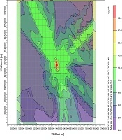
The study area was selected near the city of Tehran because, in this city, air pollution-induced by industries is a concern. The location of the stacks modeling is shown in Figure 1. The sampling of SO2 was done using a valid and reference environmental laboratory. Based on wind frequency distribution, the prevailing wind range is between 3.6 and 5.7 m/s.

AERMOD modeling domain and stack location
2. Objectives
The present study has focused on predicting SO2 concentrations induced by an oil refinery in the capital of Iran, Tehran.
3. Methods
Essential prerequisites such as source emission and meteorological data were collected from 2018 to 2019 because this information are essential for running the Aermod View software. The data were collected from documents reported by the refinery for one year. The stack sampling was carried out by environmental specialists. Amount of SO2 concentration from stacks achieved reference environmental laboratory. Table 1 describes the interested receptor specification in this study.
| No | Begin | End | Surface Roughness | Bowen Ratio | Albedo |
|---|---|---|---|---|---|
| 1 | 0 | 120 | 1 | 1.625 | 0.2 |
| 2 | 120 | 240 | 0.075 | 0.75 | 0.2 |
| 3 | 240 | 360 | 0.26 | 4.75 | 0.32 |
Receptor Specification
Data on the concentration were calculated for each stack separately. The meteorological data were collected from EMAM airport. As shown in Figure 2, the maximum frequency distribution of wind was 3.6 - 5.7 m/s, and based on Figure 3, the dominant wind direction was 45%. Table 2 describes the value of land use parameters albedo, Bowen ratio, and surface roughness, as required inputs to that were obtained through documents review and visiting the website of the oil refinery.
| Discrete Cartesian Receptors for Output | |||||
|---|---|---|---|---|---|
| Number | x-Coordinate, m | Y-Coordinate, m | Name | Terrain Elevation | Average Conc, µg/m3 |
| 1 | 536470.69 | 3933387.44 | A | 1024.00 | 42 |
| 2 | 538573.82 | 3930451.83 | B | 1012.00 | 38 |
| 3 | 541246.54 | 3934176.11 | C | 1022.45 | 85 |
| 4 | 538486.19 | 3936454.49 | D | 1037.32 | 65 |
Sector and Land Use Specification of Area Study

Diagram of wind rose for domain

Wind frequency distribution
According to the meteorological data obtained from EMAM airport station, wind roses were derived from the WRPOLT feature within the AERMET module. Due to their proximity, airport climate information can be generalized to the refinery.
The AERMOD model was run from September 2018 to September 2019, which included both cold and warm durations. Outputs were set up using 49 stacks information such as location parameter, high, diameter, sea level, and flow rate. The emission rate of each stack was calculated separately. To predict SO2 concentration, 4 locations near the refinery were selected, as receptors based on Table 1. To obtain better results, uniform receptor 25 × 25 km2 of the study area was selected as input in the AERMOD model.
4. Results
In the current study, the interested receptor was Cartesian, with a spacing of 441 receptors totally in UTM coordinates x = 538720 and Y = 3933208. in order to specify the terrain elevation in study area, the load STRM3 from USGD tab was selected. The highest values (RECTABLE) for tabular output were specified in 1, 3, 8, and 24-h to support significant contribution analyses. The air quality standard defined by the Iran environment protection agency is described in Table 3, if concentration pollutant value is higher than the standard, which can be considered as harmful to the public health.
| Pollutant | Time Period, h | µg/m3 | ppm |
|---|---|---|---|
| SO2 | 1 | 196 | 0.075 |
| 24 | 395 | 0.14 |
Iran Air Quality Standard
Regarding SO2, maximum concentration for 1-h and 24-h did not exceed 196 and 395 µg/m3. Performance measures of the model to calculate the statistical index are provided in Table 4. In the current study, the average time options of the control pathway consisted of 1, 3, 8, and 24-h. The predicted and observed concentrations of sulfur dioxide at each of the four monitoring stations were compared to verify the model performance. The NMSE index is more than 0.5 for all periods for monitoring stations, which indicates a good agreement between observed and predicted results. The fraction bias for this averaging period is between 0 and -0.5, which shows that the predicted results are close approximations of the observed results. The correlation coefficient was 0.95 and 0.92 for the two study periods. The improved coefficient for the first time was compared to the second time, which indicated a significant effect of climate condition on the dispersion pattern. The NMSE values are 0.58 and 0.65 for all periods. Using the well-known EPA statistical index, checking accuracy and the validation of the model results were performed by comparing the predicted and observed pollutant concentrations. The results of the current study indicate a good agreement between investigated values. The precision and accuracy of input parameters, such as emission and meteorological data, have an important role in the “performance appraisal” of the model. Most of the input data, such as source release parameters, location, and meteorology pathway, were obtained from target authorities (e.g., Oil Refinery Company, irimo, and NCC) (23, 24). The result of the study conducted by Paine et al. (25) for single stack evaluations about the model performance is similar to the results of this study. In this research, the aforementioned results indicate that the model performance is acceptable. Similar results are obtained by Riswadkar et al. (26) and Kumar et al. (9).
| Statistical Index | 2018 | 2019 | Period of Observation, mo | Averaging Period, h |
|---|---|---|---|---|
| CCO | 0.95 | 0.92 | 6 | 24 |
| FB | -0.38 | -0.45 | 6 | 24 |
| NMSE | 0.65 | 0.55 | 6 | 24 |
Performance Measures of the AERMOD
The comparison of observed and predicted values of SO2 concentrations for two periods is shown in Figures 4 and 5. Thus, the simulated concentration of SO2 is more close to the observed concentration. The model produces accurate predictions. As shown in Figures 4 and 5, receptor c values for pollutant concentration are higher than other values, which can be attributed to the influence of wind direction and time emission. AERMOD could appropriately predict the SO2 concentration. The impact of geographic location in different time scales on the results of simulated SO2 concentrations are described at an EPA user guide 2004. Besides, Pretty et al. showed that the performance of AERMOD was better in longer averaging time options. The developers of the AERMOD model confirmed this result (18, 27).
")
Warm time (2019)
")
Cold time (2018)
The dispersion concentration contour of SO2 derived from the model in 1, 3, 8, and 24-h averaging time, and the results are illustrated in Figures 6-9. It appears that the concentrations do not exceed the daily average national standard. As can be seen, meteorological conditions such as wind speed and the wind direction affected the amount of SO2 in the study area, which could be the cause of more spread and risk of diseases. The results of this study show that geographical and the meteorological conditions have a significant impact on SO2 plume and lower wind speed and terrain, land surface, mountains lead to the SO2 accumulation from stacks at ground levels, as reported by (28) Abdul-Wahab et al. (28). The highest concentrations of pollutants were observed nearby 53.3, 39.43 in front of the Bibishahbano mountain. The maximum estimated SO2 concentration was 66.3 µg/m3 at the distance of 5387, 3931 from the reference point in a 1-h counter. Near the stack location, there was an accumulation of pollutants and peak load, which may be due to the existence of mountains. The maximum 3-h concentration was 61.7 μg/m3 at the location of 538725, 3931936. In this situation, as similar to 8-h, counter pollutants domain was less spread. Output values of SO2 concentration predicted from oil Refinery indicated that pollution is spreading mostly from North West to South East direction according to the predominant wind, as shown in Figure 2.

SO2 dispersion in 1-h

SO2 dispersion in 3-h

SO2 dispersion in 8-h

SO2 dispersion in 24-h
As shown in the above figures, the the maximum predicted concentration of SO2 was 1, 3, 8, and 24-h for each month of the year. The geographical and meteorological conditions affect SO2 concentrations. In this study, the influence of SO2 emission from refinery stacks was simulated by the Aermod View dispersion model. The results of this study are not as good as those reported by Yassin et al. (29). Concentration values of SO2 were lower than limits set by the Iran Environmental standard in all time intervals. This indicates that the stack’s emission of SO2 has no significant effect on the quality of ambient air in this region.
| Result Summary of SO2 Concentration | |||||
|---|---|---|---|---|---|
| Averaging Period, h | Rank | Peak, µg/m3 | X | Y | Peak Date |
| 1 | 1st | 66.27 | 538725.45 | 3931936.05 | 5/8/2019, 11 |
| 3 | 1st | 61.69 | 538725.45 | 3931936.05 | 5/8/2019, 12 |
| 8 | 1st | 36.12 | 538725.45 | 3931936.05 | 7/13/2019, 16 |
| 24 | 1st | 12.73 | 538725.45 | 3931936.05 | 4/24/2019, 24 |
Model Output
The results of SO2 dispersion in the study area are shown in Table 5. The maximum concentration of pollutants was 66.27 μg/m3 on 05/08/2019 in a 1-h counter. The minimum concentration was 6.1 μg/m3 on 02/28/2019 in the monthly counter.
5. Discussion
This study presented the distribution of SO2 from 49 refinery stacks using the AERMOD model. Although the simulation indicated that the concentrations of SO2 were very low, it could have effects on the population health, environment, long-term biological accumulation in organisms, which chemical compounds and air pollutants absorb through different routes. The effect of terrain was shown for SO2 dispersion. It also appeared that the concentrations of SO2 pollutants are relatively high and accumulated in front of the mountain for all days during the study period, compared to other locations and periods. Further, a good agreement was observed between the predicted and observed SO2 concentrations using the AERMOD model evaluation. The measurements showed that the wind speed and direction play a significant role in the dispersion SO2, that the dominant wind direction was from the northwest and maximum concentrations occurred in the North and West and when air pollution dispersion spread to south and east according to wind rose.
5.1. Conclusions
Various parameters can affect the SO2 dispersion from oil refinery stacks. In addition to characteristics of source emission, local meteorological parameters, and geology, which are important inputs for air dispersion modeling as reported by Ozkurt et al. (30). This study prepared a useful approach to decision making about air pollution management in the oil refinery. It can be useful where information on air quality are not sufficient.
