1. Background
The world faced an international public health emergency in late December 2019 that started in Wuhan, China (1) numerous cases appeared rapidly in Asian countries and spread to other continents, which led to on March 11, 2020, the World Health Organization declared it a global pandemic, the main cause of which was severe acute respiratory syndrome coronavirus 2 (SARS-CoV-2) (2). Simultaneously with the wide spread of COVID-19 in the world, the need to study this communicable disease from a geographical point of view to answer different needs and questions was highlighted (2). This is due to the fact that COVID-19 disease has unknown features (2), Many climatic and spatial variables can effect on changes in the pattern of COVID-19 occurrence (3). Geography defines spatial, territorial, locational, and landscape aspects (4).
One of the most important research methods in this aspect of the pandemic period is spatial analysis (5). Spatial analysis that considers geographical development includes a set of statistical methods and trends (6, 7) that, by examining the incidence and prevalence of diseases, prepares them in the form of geographical maps, and the result is an explanation of dispersion (8). Thus, disease mapping has become necessary in public health (9).
Disease monitoring provides the basis for conducting research programs on the cause of the disease and evaluating early public health interventions (6). The incidence, prevalence, and deaths of diseases change over time (10). Temporal statistics are used to identify time trends. The temporal trend is determined by the annual percent change (APC) (11). Since the disease has spread rapidly in many regions, the pandemic has become a challenge for health decision-makers and Health service managers (12). So understanding of the spatiotemporal dynamics of COVID-19 is crucial for the prevention of incident cases. Because it helps policymakers reduce the prevalence rate and spread of disease (3, 13). According to the climate variation and socioeconomic differences in different countries, spatial analysis can determine disease distribution worldwide (14, 15) and also help comprehend patterns of incidence, mortality, morbidity, and burden of COVID-19 (16).
2. Objectives
In this regard, in the present study, we aim to understand the geographic pattern and temporal trend of the 2019 Coronavirus disease incidence worldwide to strengthen healthcare services and actions in high-risk regions. Also, this study provides information about morbidity, mortality, and recovery of COVID-19 disease from October 1, 2019, until June 30, 2021.
3. Methods
3.1. Design and Type of Study
This ecological study was designed as a mixed exploratory study. In exploratory studies, investigators discover and describe patterns of disease. The mixed study indicates that both temporal trends (Time trend) and spatial patterns (multiple-group study) are investigated (6, 17).
3.2. Target and Study Population
The target population consists of all patients infected with COVID-19 worldwide. The study population includes countries where information on morbidity, mortality, and recovery was available from October 1, 2019, until June 30, 2021.
3.3. Data Collection and Data Source
In this study, three main types of data sources were used. The data on the population at risk of COVID-19 were obtained from the World Bank website (18), and for obtaining the number of COVID-19 patients from October 2019 until June 2021, each country used CDC and WORDOMETER websites (19). Another source contained patients’ geographical coordinates data obtained from the georeferenced layer of Google Maps in each country.
3.4. Statistical Analysis
In this study, descriptive analysis of data was performed to determine the CIR, CFR, and CRR of COVID-19 in each county from October 1, 2019, until June 30, 2021. Data analysis was done with ArcGIS, Joinpoint, and SPSS software at a 0.05 significance level.
3.5. Cumulative Incidence Rate, Case Fatality Rate, and Case Recovery Rate Measurements
In order to compute the cumulative incidence rate of COVID-19, the number of newly diagnosed cases during a specific period was divided into the total population at risk during the beginning of the period in 106 individuals (20). CIRs measure the risk of developing the disease (21). Case fatality rate (CFR) and case recovery rate (CRR) were specified as the proportion (percent) of people who died and recovered from COVID-19 among all individuals diagnosed with COVID-19 over a certain period of time at the global level, respectively. The CFR is a measure of the severity of mortality or virulence of a disease and is sometimes used to predict the prognosis of the disease. The CRR reflects the quality of care and the strength of the health system (17, 22).
3.6. Temporal Trend
With the Joinpoint regression program version 4.7.0.0, the cumulative number of new cases, CFR, and CRR were calculated monthly and annually in order to evaluate the temporal trend of COVID-19. In this study, CIR, CFR, and CRR were dependent variables, and months and countries were independent variables. In order to compute the average annual percentage change (AAPC) and the annual percentage change (APC), we employed the natural log-linear model according to the Poisson distribution of dependent variables. The Grid search method was used to calculate the joint points where the incidence rate changes drastically (10). The Monte Carlo method estimated the P-value with 4499 iterations. The precision of models was examined by the sum of squared errors (SSE) and Bayesian information criterion (BIC). Regression line slope changes and the estimated APC-AAPC values were obtained for the annual trend of COVID-19 as well as; in order to evaluate the seasonal trend of COVID-19; the incidence rate was calculated by month. Finally, monthly slope alterations of trend, joinpoint times, and amounts of APC and AAPC were computed by joinpoint regression analysis.
3.7. Spatial Pattern Analysis and Cluster Identification
A spatial pattern for COVID-19 was determined by mapping the CIR, CFR, and CRR of each country using ArcGIS software version 10.8.
Global Moran's I was used to designate spatial autocorrelation of COVID-19 in the world. The value of global Moran's I is variable from -1 to 1 (23). The values near +1 show clustered distribution, values near -1 show dispersion, and zero indicates the random distribution of COVID-19 in the area under study (23).
In the next step, Anselin Local Moran's I was used to define the low-risk and high-risk cluster locations of COVID-19. This index focuses on the central polygon and compares it with the surrounding areas. Anselin Local Moran's I split polygons into five categories, containing low-high, high-low, low-low, high-high, and not significant (10). According to this category, in the H-H cluster, firstly, the incidence of disease in these areas is higher than the average incidence of disease in the entire study area, and secondly, the incidence of disease in this area and the surrounding neighbors is high, which is called a hot spot (10). The L-L cluster occurs when the incidence of disease in that cluster is lower than the world average, and the incidence of disease in the central polygon and surrounding countries is low, which is called cold spots[a1]. This index also identifies outliers, which are identified as H-L and L-H (10).
In order to indicate more precise clusters of COVID-19 in the world, an optimized hot spot analysis (OHSA) was employed. This method, according to the Getis-Ord Gi*, with the optimization of distance band for determining hot and cold spots (24). Using incremental spatial correlation, OHSA automatically selects the optimal bandwidth value at which spatial autocorrelation and clustering intensity are maximum and then uses it as an analytical scale for the Getis-Ord Gi * statistic (24). This will show the output's best possible results to identify hot and cold spots. OHSA demonstrates results at 90%, 95%, and 99% confidence levels (24).
This study is approved under the ethical approval code of IR.SBMU.RETECH.REC.1398.876.
The webpage of the ethical approval code is: (ethics.research.ac.ir/ProposalCertificateEn.php?id=125693)
4. Results
4.1. Descriptive
In the present study, the average cumulative incidence rate was 1077 per 106 individuals. Also, the average case recovery rate and average case fatality rate were respectively %72.81 and %3.21 from the outbreak of the epidemic in October 2019 until the end of June 2021. The table in the Appendix 1 shows the CIR-CFR-CRR values of all countries in the world every month.
4.2. Spatial Pattern and Cluster Identification
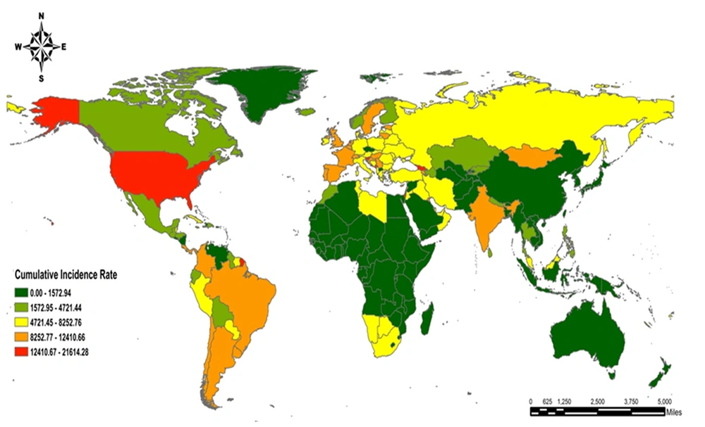
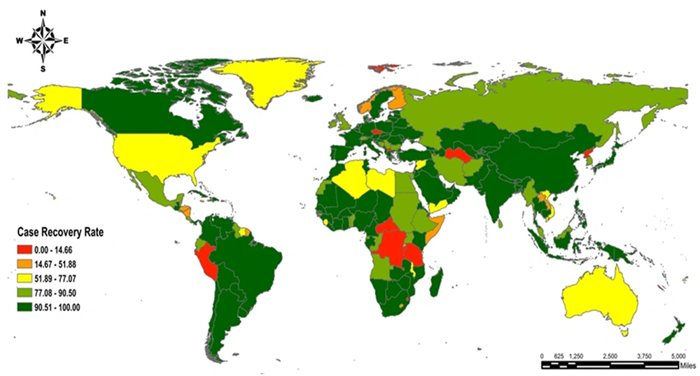
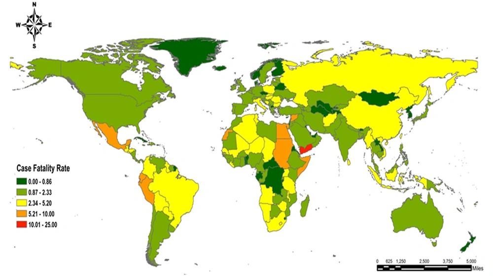
Spatial patterns of CIR, CFR, and CRR, which were in association with COVID-19, have been declared in Figures 1-3 from the onset of the epidemic in October 2019 until the end of June 2021, and then the zoning of the disease was drawn in GIS environment.
Overall, given the CIR, some parts of North America and the next level, the entire continent of South America, whole parts of Europe apart from Eastern Europe, and a few areas of Eastern and Southern Asia reported the highest CIR, respectively. On the other hand, the lowest CIR is recorded in the entire continent of Australia and Africa except for South Africa and a few northern regions of this continent, some of the continents of Asia and Northern America. The list of countries with the highest CIR consists of Seychelles (CIR = 21614.284), Montenegro (CIR = 20506.762), Andorra (CIR = 19615.608), Gibraltar (CIR = 16330.770), Bahrain (CIR = 16138.812) whereas Micronesia (CIR = 0.182), Vanuatu (CIR = 1.302), Samoa (CIR = 1.511), Western Sahara (CIR = 1.674), Tanzania (CIR = 2.288) are five cities with the least CIR (Figure 1). Considering countries that are more affected by the epidemic and reported the highest total case, CIR could be mentioned as follows: USA (CIR = 13151.648), UK (CIR = 11144.975), India (CIR = 11144.975), Brazil (CIR = 10024.574) and Russia (CIR = 5054.579911). As for Figure 1, the USA has first place, India, Brazil, and the UK is in second place, and Russia is in third place in CIR.
Regarding Figure 2, the highest case recovery rate was relevant to Europe and West America, while areas of Middle and Eastern Africa and the entire continent of Australia, and some parts of northern America in the next level had the least CRR. By and large, CRR has been reported to be above 77% in about 80% of countries. For example, CRR was 100% in countries with less than 50 cases. Nevertheless, CRR was reported to be more than 90% even in countries in which the incidence rate passed 200,000. Having said that, CRR was too low in some countries, such as Martinique, with the lowest CRR worldwide and approximately 41 thousand incidences. New Caledonia had the slightest CRR after Martinique, with 0.99% of CRR and about 6 thousand incidences. Other countries with less than 5% of CRR include Guadeloupe and Burundi. CRR values for countries with the highest reported total cases are as follows: USA (CRR = 75.882), India (CRR = 97.766), Brazil (CRR = 95.360), UK (CRR = 80.688), and Russia (CRR = 89.130).
In view of CFR, large areas of Africa, Asia, and South America showed the highest rate, while some areas of North America, Europe, and Australia showed the least. The highest CFR at the time of study is assigned to Vanuatu, which had one death from 4 infected cases and Yemen had the second place with 9 thousand incidences (CFR = 18.88%). The third place of CFR pertains to Peru, with an incidence rate of more than 2 million (CFR = 9.175%); in addition, Mexico and Sudan had the fourth and fifth place with approximately 7.5% of CFR, respectively. The lowest CFR respectively pertains to Laos (CFR = 0.075%), Singapore (CFR = 0.084%), Bhutan (CFR = 0.115%), Faroe Is (CFR = 0.182%), and Burundi (CFR = 0.232%) (Figure 3).
4.3. Anselin's Local Moran’s I Results
The results of Global Moran’s I analysis show that the value of this index was measured at 0.159, which indicates the intensity of autocorrelation and the very high tendency of COVID-19 disease for clustering. The obtained Z score = 12.11 and P-value < 0.001 demonstrate that the disease spatial autocorrelation rate is significant even at the confidence level of 0.99. The figure in the Appendix 2 provides information about the gained results of analyzed Global Moran’s I.
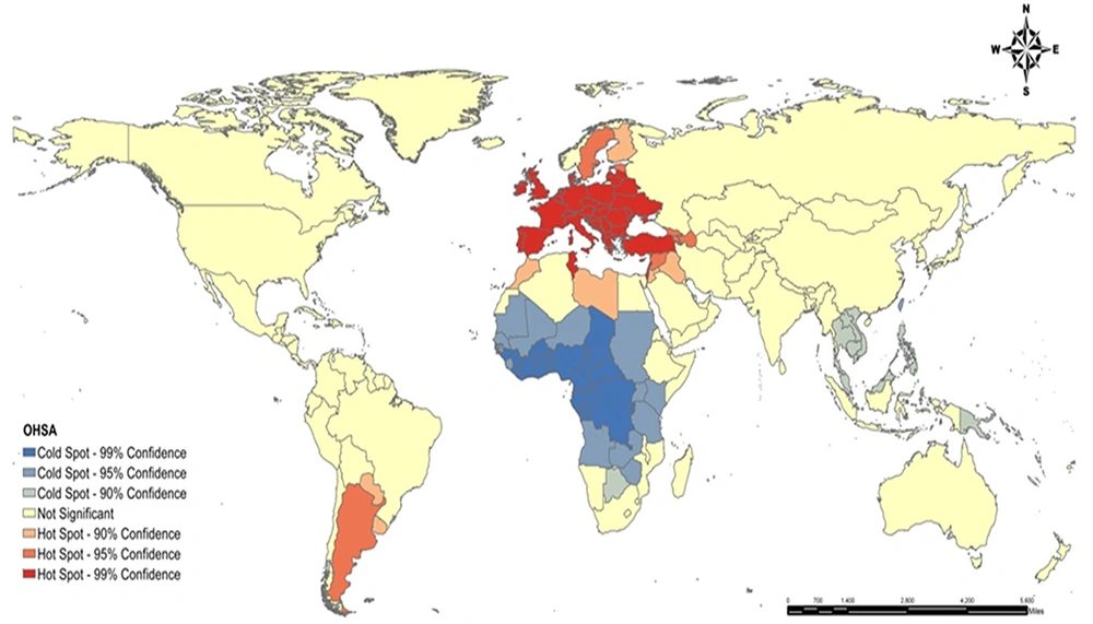
4.4. Optimize Hot Spot Analysis Results
The optimal value of bandwidth is estimated to be 2411.332 kilometers based on the OHSA method. This indicator identified hot spots in countries that are mostly located in the south and west of Europe and west of Asia. These countries include Belgium, Israel, France, Netherlands, United Kingdom, Spain, [a1] Portugal, Turkey, Greece, Poland, and Tunisia in Africa (99% of confidence level), Armenia, Azerbaijan, Georgia, Argentina, Syria, Sweden (95% of confidence level) and Iraq, Jordan, Libya, Morocco, Paraguay, Uruguay, Finland (90% of confidence level).
Moreover, cold spots are recorded in countries of Western Africa and Middle Africa such as Zaira, Congo, Gabon, Chad, Cameroon, Nigeria (99% of confidence level), and other countries like Mauritania, Mali, Niger, Sudan, Kenya, Angola, Zambia (95% of confidence level) and New Guinea, Laos, Vietnam, Cambodia, Thailand, Malaysia, Brunei, Taiwan, Botswana (90% of confidence level). With an overall look at the zoning of clusters, a majority of hot spots are located in Europe, southern and western parts of it in particular, central and western parts of Asia, and to a lesser extent, some countries of South America and North Africa. On the other hand, cold spots are located in East, West, and Central Africa and some parts of South East Asia (Figure 4).
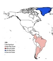
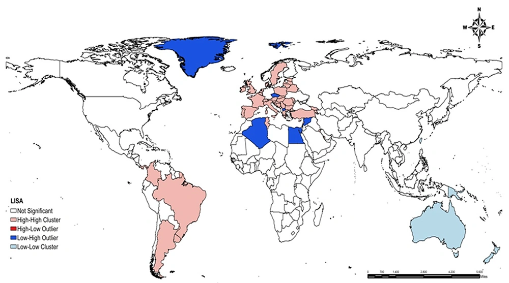
As regards the results of Anselin's local Moran’s I, the High-High cluster consists of some countries such as Brazil, French Guiana, Colombia, Uruguay, and Argentine in South America and Sweden, Ireland, United Kingdom, France, Spain, Turkey, Tunisia, Poland, Belarus, Estonia, Latvia Ukraine, Switzerland, Italy, Romania, Bulgaria, Greece, Georgia, Armenia in southern and western Europe and central and west Asia. It declares the spatial clusters of high values and high risk of incidence in these regions. Indeed, the incidence rate in these countries is more than the global average value; in addition, they are surrounded by countries with a high outbreak.
On the other hand, Australia was identified as a Low-Low cluster which reveals the spatial cluster of low values and low risk of this disease in these regions. Firstly, the incidence rate is less than the global average. Secondly, they are surrounded by countries with low outbreak (Figure 5).
4.5. Time Trend Results
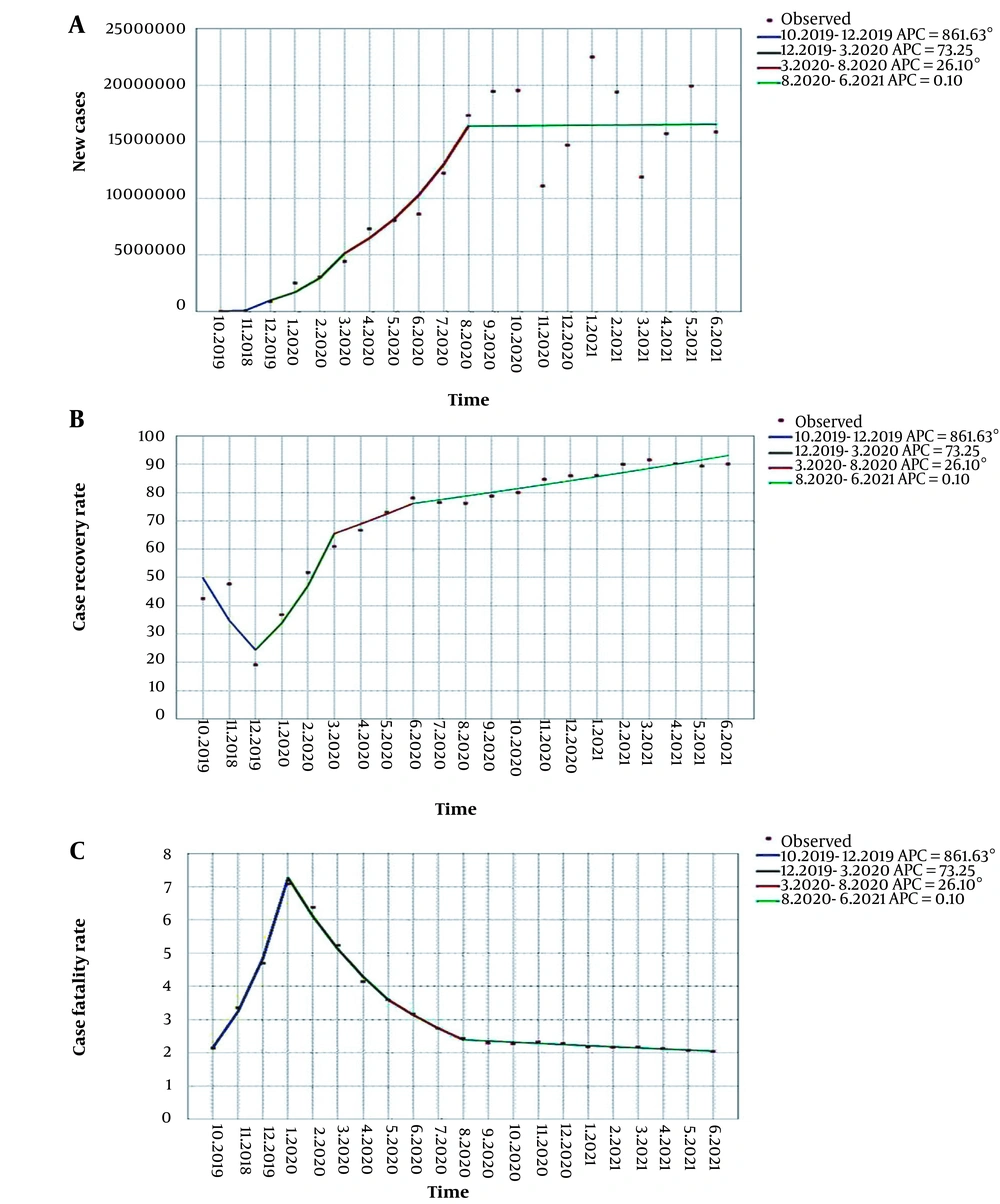
Time trend results of new cases, case recovery rate, and case fatality rate were analyzed by joinpoint regression on a monthly basis and are shown in Figure 6 and Table 1.
| Number of Graph-related | The Time Frame of the Trend | APC | P-Value | AAPC | P-Value | ||
|---|---|---|---|---|---|---|---|
| Point Estimate | 95% CI | Point Estimate | 95% CI | ||||
| 7(A) | 10.2019 - 12.2019 | 861.63 | 370.6, 1865.2 | < 0.001 | 44.4 | 27.3,63.8 | < 0.001 |
| 12.2019 - 3.2020 | 73.25 | -15.2,254.0 | 0.1 | ||||
| 3.2020 - 8.2020 | 26.10 | 0.6,58.1 | < 0.001 | ||||
| 8.2020 - 6.2021 | 0.10 | -5.3,5.8 | 1.0 | ||||
| 7(B) | 10.2019 - 12.2019 | -30.08 | -35.5, -24.2 | < 0.001 | 3.2 | 1.5,4.9 | < 0.001 |
| 12.2019 - 3.2020 | 39.06 | 28.3,50.7 | < 0.001 | ||||
| 3.2020 - 6.2020 | 5.16 | -3.0,14.0 | 0.2 | ||||
| 6.2020 - 6.2021 | 1.69 | 12,22 | < 0.001 | ||||
| 7(C) | 10.2019 - 1.2020 | 49.63 | 45.1,54.3 | < 0.001 | -0.3 | -1.3,0.8 | 0.6 |
| 1.2020 - 5.2020 | -16.10 | -18.6, -13.5 | < 0.001 | ||||
| 5.2020 - 8.2020 | -12.73 | -17.9,0.72 | < 0.001 | ||||
| 8.2020 - 6.2021 | -1.52 | -2.0, -1.1 | < 0.001 | ||||
Figure 6A and Table 1 illustrate the time trend of new cases in each month and year. As for the gained results, differentiation of disease incidence had been on the rise between October 2019 (10.2019) and June 2021 (6.2021), and the average (AAPC) increased by 44.4% per year (P < 0.001). Although a joinpoint was observed in 12.2019 and new cases changed substantially in this time period, the frequency of new cases increased dramatically between 10.2019 and 12.2019 (APC = 861.63%), notwithstanding the severity of disease incidence decreased from 12.2019 to 3.2020 (APC = 0.1%). Furthermore, there was a new significant joinpoint in 8.2020, although the incidence of new cases of the disease has reached stability and is increasing at the same rate in the period between 6.2021 and 8.2020 (APC = 0.1%).
Temporal analysis with joinpoint regression models fitted to new cases of COVID-19 in the world during COVID-19 During Oct 2019 to Jun 2021. (A) Temporal analysis with joinpoint regression models fitted to the case recovery rate of COVID-19 in the world during during Oct 2019 to Jun 2021. (B) Temporal analysis with joinpoint regression models fitted to case fatality rate of COVID-19 in the world during Oct 2019 to Jun 2021. (C) *Indicates that the annual percent change (APC) is significantly different from zero at the alpha = 0.05 level
The time trend of the case recovery rate in each month and year is demonstrated in Table 1 and Figure 6C. CRR had risen substantially from the onset of the outbreak until June 2021 (6.2021), and the average (AAPC) increased by 3.2% per year (P < 0.001). But a joinpoint was observed in 12.2019, and the CRR shifted significantly in this time period, so this progression experienced a considerable drop between 10.2019 and 12.2019 (APC = -30.08%), whereas the APC increased from 12.2019 to 3.2020 (APC = 5.16%). Thus, there was another joinpoint in 6.2020, albeit CRR increasing progression seems to be more stable between 6.2020 and 6.2021. It soared dramatically, but even so, the velocity of this increase has plunged down (APC = -1.69%).
Table 1 and Figure 6C declare the time trend of the case fatality rate in each month and year. CFR has decreased since the onset of the epidemic, and this falling progression continued until June 2021 (6.2021). It averagely dropped by -0.3% per year (AAPC), which was not considerable (P > 0.05). Although a joinpoint was observed in 1.2020 and CFR varied substantially as a consequence of this joinpoint, this indicator had a significant rise between 10.2019 and 1.2020 (APC = 49.63%). Despite that, it fell considerably between 1.2020 and 5.2020 (APC = -16.10%) and continued decreasing with a lower speed in the time period between 5.2020 and 8.2020 (APC = -12.7%). Hence the second joinpoint occurred on 5.2020, and ultimately, in the period of 8.2020 - 6.2021, it significantly reached its lowest growth rate (APC = -1.5%). The third joinpoint arose on 8.2020.
5. Discussion
From the pandemic's beginning in October 2019 until June 2021, the average case fatality rate was estimated at 0.031. Although CFR only increased in the first four months of the pandemic, it decreased from May 2020 until June 2021. This falling process may be due to countries' access to diagnostic tests, which has increased recently. This theory is consistent with a study in Illinois which states that raw CFR decreases in all regions and age groups during the development of diagnostic tests (25). This study also showed an increase in CRR. There has been no specific medicine for this disease, even though various combinations of drugs and therapies are utilized, most of which are supportive and symptomatic. As for the pneumonia-like symptoms of COVID-19, early diagnosis and controlling these symptoms results in valuable findings and a better-soaring improvement rate (13, 15, 26).
The results of this study revealed that the highest CIR is recorded in America and Europe. Perhaps the reason is that more diagnostic tests are taken in these developed areas (27).
Global Moran's I = 0.159 and obtained Z score and P-value showed that spatial autocorrelation rate and tendency to spatial clustering of COVID-19 disease is very high. This finding develops the assumption of the possible association of environmental risk factors with COVID-19, such as temperature, humidity, hours of sunshine, topographic and built environment, etc. (28). Several studies have shown that temperature and humidity are the main factors that affect SARS-CoV-2. Studies are compromised on the inverse correlation between temperature and humidity in global SARS-CoV-2 transmission. COVID-19 has sessional variations; however, vague results about the effect of humidity on SARS-CoV-2 transmission were obtained with reference to other meteorological factors such as air pollution, wind speed, etc., analyses performed in local areas (29).
We can mention the results of a study that was held in 16 African countries in view of recording cold spots in Africa. It stated that higher temperatures and humidity decrease the new daily cases and fatality rate of the COVID-19 outbreak. Therefore, these factors minimize the daily incidence and mortality from COVID-19 epidemics in African countries (30).
With an overall look at the zoning of clusters, it can be concluded that most hot spots are located in Europe, Asia, and to a lesser extent, some countries in America and Africa. On the other hand, cold spots are located in Africa and some South East Asia. Finding hotspots in developed areas could be associated with high population density, a higher proportion of the elderly population (31), high population movement via road, rail (9). Despite that, recording hot spots in regions with lower socioeconomic status, such as some parts of Asia, indicates poor access to health facilities and a higher risk for disease incidence as a consequence (15, 32).
Another result of the present study is a significantly increasing progression of disease incidence between Oct 2019 (10.2019) and June 2021 (6.2021). It had the highest growth rate in the first months through the last ten months of evaluation demonstrated the lowest growth rate. The growth rate was some have stable in this period. The high growth rate at the beginning of the pandemic outbreak could be due to a dramatic increase in patients in Wuhan, China, rapid transmission to other countries, and failure to discover suitable methods to diagnose and treat the disease (33).
The drop in the speed of disease rate may have pertained to the observation of health protocols, personal hygiene, and the use of protective equipment such as face mask and shield, gown, gloves, glasses, and N95 respirator, especially in hospital environments, proper ventilation, hand washing with soap and water or alcoholic disinfectant after contact with any contaminated surface (34), a social distancing that has affected the pattern and rate of population movement, purposeful implementation of local quarantines (35), reduction of gatherings, social events and group meetings (34), use of efficient diagnostic tools such as rapid and large-scale tests which play an essential role in patient management and reducing the rate of a disease outbreak (36) and most importantly, vaccination which is essential for infection prevention, controlling disease prevalence and reducing its recurrence rate, etc. (37).
The average case recovery rate had been plummeting in the first three months of the epidemic outbreak significantly and, after that, soared until the end of the period of study. Moreover, CFR had been increasing for the first five months of the epidemic, though it started a decreasing progression which continued until June 2021 (6.2021). This increasing process of recovery rate and reduction of CFR may be due to the strengthening of the immune system and promotion of self-care by striving for a healthy lifestyle and consuming adequate nutrients (38, 39), paying efforts to accelerate the development of treatment for COVID-19 by reusing antiviral drugs which are previously produced and approved by the FDA or currently assessed for other viral infections and combining these drugs with new technologies. These treatments aim to reduce the SARS-CoV-2 infection burden in patients, decreasing the severe symptoms and slowing down the COVID-19 improvement (40-42). For the most part, timely diagnosis and early treatment of infected cases are the first steps to winning this battle (13).
5.1. Conclusions
As regards the specific spatial pattern of fatality and recovery rate of COVID-19, it seems essential to consider spatial conditions and environmental factors which are related to the incidence and fatality of COVID-19 in different regions, as do the necessity of upgrading the care system in high-risk areas, in order to have better management and control of the pandemic and optimal function in early diagnosis, proper treatment, and high vaccination coverage.
