
1. Background
The liver is the most important internal organ of the body, which plays a primary role in the body's metabolism. Patients with liver disease are increasing due to risky lifestyles such as excessive consumption of alcohol, inhalation of harmful gases, unhealthy diets, and excessive use of drugs. Liver cancer is the third leading cause of death worldwide. The concern is that liver cancer is not easily diagnosed, and there are no clinical signs in the early stages because the liver can maintain its normal function despite some parts being damaged. Therefore, timely diagnosis of liver cancer is crucial in treating these patients and increases their survival rate (1).
Monitoring is done to check the health and physiological status of people. The goal of monitoring is early detection and reduction of disease-related mortality. Achieving this goal is usually possible through early diagnosis. Several ways can be used in examining patients with liver disease. Ultrasound is one of the methods recommended for patient follow-up as a non-invasive, easy-to-use, real-time, and relatively low-cost technique (2).
Although medical science has made many advances, detecting liver nodules by ultrasound is still difficult. The timely diagnosis of this disease is directly related to the sonographer's experience. As a result, researchers are trying to design a system to help them with the diagnosis of cancer masses. Some of these models include learning machines and neural networks. The main purpose of these models is to determine the effective variables, relations between them, prediction, and estimation, which are very important in medicine (3).
Images help to visualize changes in liver tissue along with pathology. A radiologist described the two stages of the liver:
(1) A normal liver has a smooth, homogeneous surface without prominent nodules or depressions, well-defined borders, fine parenchymal echoes, normal size, and normal portal vein diameter (4).
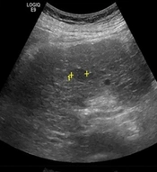
(2) On grayscale ultrasound, Hepatocellular Carcinoma (HCC) typically appears as hypoechoic lesions, especially when they are small. In some cases, increased echogenicity due to adipose degeneration may be observed. Occasionally, hypoechoic nodules may represent hyperechoic lesions, suggesting the development of HCC in dysplastic nodules (5).
Computer-aided diagnosis systems for liver disease can assist clinicians in making decisions by considering the liver surface, quantifying diagnostic features, and classifying liver disease. The liver deformity can be quantified by evaluating the texture of ultrasound images. Table 1 summarizes studies performed on computer-aided diagnostic systems using liver ultrasound images (4).
Table 1.
Summary of Previous Studies on Computer-aided Diagnostic Systems Using Liver Ultrasound Images
| Authors | Liver Image Type (No. of Patients) | Feature Extraction Methods | Feature Selection Strategy | Classifier | Classification Accuracy (%) |
|---|---|---|---|---|---|
| Kyriacou et al. (6) | Normal (n = 30); Fatty (n = 30); Cirrhosis (n = 30); HCC (n = 30) | GLDS, RUNL, SGLDM, FDTA | - | k-NN | 74.2; 77.5; 78.3; 70.8; Combination of RUNL, SGLDM, FDTA:80 |
| Wu et al. (7) | Normal (n = 90); HCC (n = 166) | GLCM, WT, Gabor WT | Genetic algorithm | k-NN, fuzzy k-NN, PNN, SVM | Fused feature set: 96.6 |
| Bharti et al. (4) | Normal (n = 48); CLD (n = 50); Cirrhosis (n = 50); HCC (n = 41) | GLDM, GLCM, Ranklet transform | HFS | k-NN, SVM | 95.2; 92.3 |
2. Objectives
It is noticed from the summary of research papers that textural feature extraction and feature selection methods have a significant role in computer-aided diagnostic systems. This study uses a gray level co-occurrence matrix (GLCM) to extract textural features from discrete wavelet transform (DWT) images. After that, t-test and sequential forward floating selection (SFFS) are applied to improve the resulting classification performance.
3. Methods
3.1. Database
In this study, a database of 400 liver ultrasound images was clinically obtained in the DICOM format. They included 200 normal livers and 200 hepatocellular carcinomas. The ultrasound images were collected from the Cancer Imaging Archive and Kaggle websites. Ultrasound images of hepatocellular carcinoma patients had 3 × 720 × 960 sizes obtained from a GE (General Electric, USA) ultrasound machine in 2013 and labeled by a radiologist (8, 9). Moreover, ultrasound images of normal people were collected from the radiology department of Geneva University Hospital, Switzerland (10, 11).
3.2. Preprocessing
Since grayscale conversion is used in medical practice for computer-aided diagnosis, the images were first converted from RGB to grayscale, and then the contrast was normalized. The best-known color model is RGB, derived from the words red-green-blue. As the name implies, this model represents colors by individual values for red, green, and blue. Three integer values from 0-255 are used to indicate each color. Grayscale is the simplest model because it defines colors with only one component: brightness. However, they are widely used in image processing because using a grayscale image requires less space and is faster, especially when complex calculations are involved. The best conversion method is the luminance method, as indicated in Equation 1 (12).
We used morphology and image masking operations to remove the foreground and define image boundaries.
Denoising aims to improve image data by reducing noise or suppressing unwanted artifacts. In this study, a median filter was utilized to remove noise. Median filtering is broadly utilized in image processing because it preserves edges while removing noise. The median filter is a technique wherein it effectively distinguishes out-of-range noise from legitimate image features such as edges (13, 14).
The idea of mean filtering is to replace each pixel value in an image with its neighbors' mean value, including itself. This has the effect of eliminating pixel values that are not representative of their surroundings. The image processing function of the median filter can be expressed as follows:
where M is the total number of pixels in the neighborhoods, N, g(i, j) is the processed image, and f (k, l) is the input image (15).
Cropping an image means removing unwanted areas or unnecessary information and defining a Region of Interest (ROI). This improves the accuracy and speed of processing and limits the possibility of error by selecting only the most informative regions (16). In this study, images with 64×64 pixel resolutions were obtained after cropping.
3.3. Feature Extraction
3.3.1. Discrete Wavelet Transform
Discrete wavelet transform (DWT) is one of the most effective tools for image compression. It is to decompose the image hierarchically into a multi-resolution pyramid. Application of DWT to a two-dimensional image corresponds to image processing by a two-dimensional filter in each dimension. This filter divides the input image into four non-overlapping sub-bands with multi-resolution: HL, LL, LH, and HH. The DWT provides very good compression properties for many image classes. In this study, dB8 was used for decomposition. The GLCM characteristic values were calculated from the approximate, horizontal, vertical, and diagonal components of the first decomposition level, as shown in Figure 1 (16).
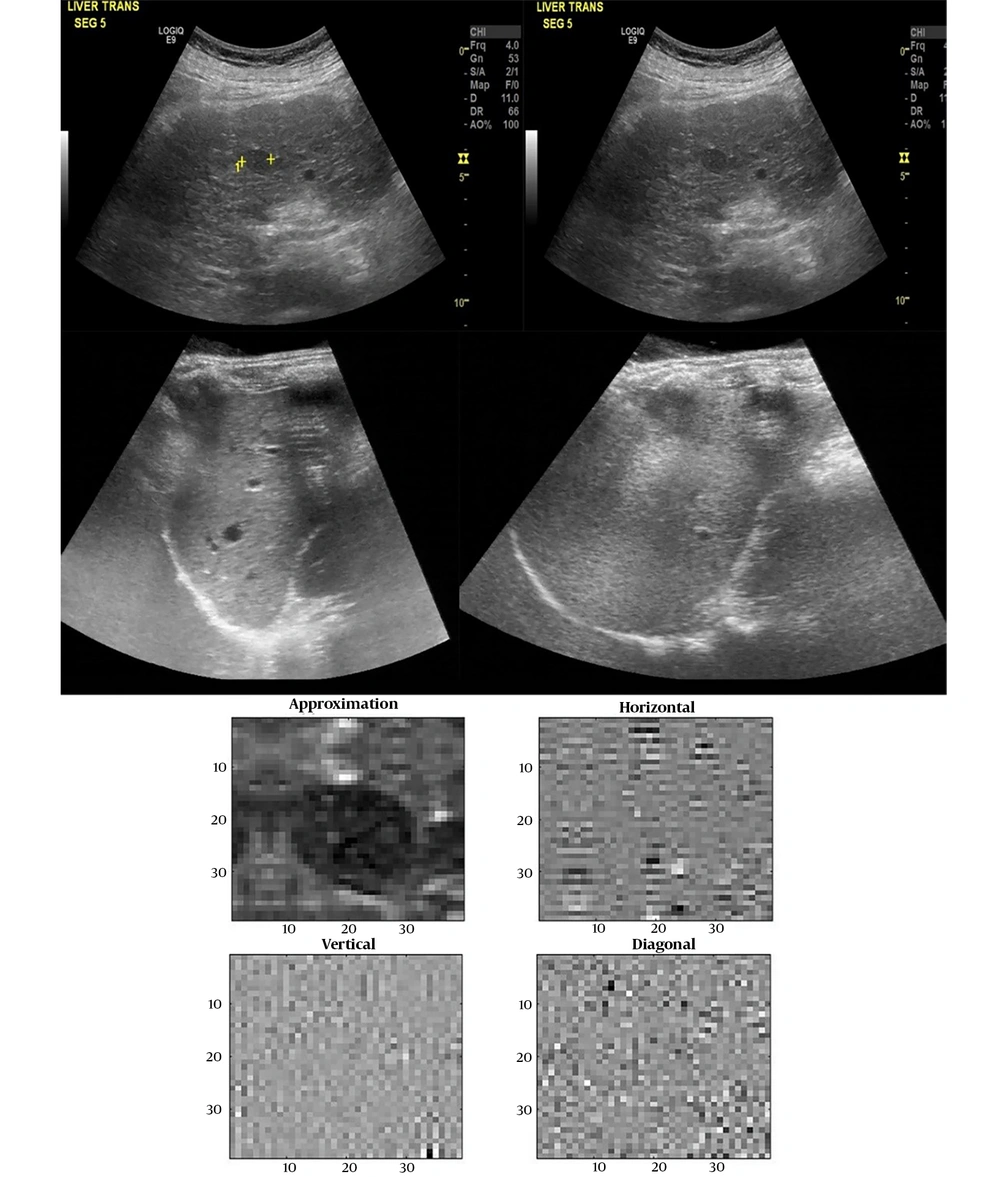
Figure 1.
Ultrasound image of normal and hepatocellular carcinoma livers (above) and discrete wavelet transform image (bottom)
3.3.2. Gray Level Co-occurrence Matrix
The GLCM is one of the most well-known texture analysis techniques for evaluating image properties related to second-order statistics, considering the spatial relationship between two adjacent pixels, where the first pixel is the reference pixel and the second pixel is the adjacent pixel. The GLCM is calculated based on two parameters: The relative distance d between a pair of pixels, measured as the number of pixels, and the relative orientation φ. With relative distance d = 1 and relative orientation φ = 0, the coordinates (x, y) are [0, 1]. After setting the orientation, we configured the number of graycomatrix to scale the image with the number of gray levels parameter and scales the values of graycomatrix with the gray limits parameter. In this study, the grayscale matrix using the number of gray levels was 32, which means 25 or 5 bits, and it uses the minimum and maximum grayscale values in the input image as constraints (17).
In the next step, the image features were extracted to measure the textural properties of images and use them for classification. The extracted features should be able to produce the maximum similarity between samples from the same category and the maximum difference between samples from different categories to achieve the best classification efficiency. Texture differences between malignant tumors and normal tissue also cause pixel-wise intensity changes.
Since malignant lesions have irregular tissues unlike normal tissues, stromal-derived features are also important for gray levels to occur. A GLCM provides information about the relationship between values of adjacent pixels in an image. The number of rows and columns in the GLCM equals the number of gray levels in the image. If the number of gray levels in an image is D, then the dimension of the GLCM is D×D. The element G(i.j|Δx.Δy) of this matrix is the number of repetitions of the relationship between 2 pixels separated by a spatial distance (Δx.Δy) where one of the pixels has gray level i and the other one has gray level j.
After calculating the matrices, 22 features were calculated for every image from the GLCM, and their average was used as GLCM texture features. These features consisted of autocorrelation, contrast, correlation, cluster prominence, cluster shade, dissimilarity, energy, entropy, homogeneity, maximum probability, variance, difference entropy, difference variance, sum average, sum variance, sum entropy, information measure of correlation 1, information measure of correlation 2, inverse difference (INV), inverse difference normalized (INN), and inverse difference moment normalized (18).
Eventually, 110 features were extracted from most of these images via the GLCM technique. Then, each of these features was normalized by Equation 3:
3.4. Feature Selection
Since it is impossible to precisely determine which factors are effective and directly related to the required task in complex problems, many factors must be extracted as features. In this case, the data dimensions increase significantly, resulting in a larger number of coefficients for the classifier or regression algorithm used in decision-making. This can make it challenging to generalize the algorithm, which is the main difficulty in designing a model. On the other hand, the feature extraction process may extract features that do not provide useful information for solving the problem, are probably repetitive, will not add new information to the problem, and may even be associated with noise, compromising the analysis.
Dimension reduction techniques are used to solve these issues and reduce the number of features. Dimension reduction methods include feature mapping and feature selection, each reducing the number of features with a single approach. The feature mapping approach maps features from one space to a new space; in other words, features are combined to create new features, and the number of these features is reduced compared to the original space. In feature selection methods, several features are selected based on a set of criteria to reduce the number of features (19).
This study decided to use both vector and scalar feature selection methods to speed up feature selection based on class clauses and provide optimal feature subsets. Therefore, the selection of scalar features was performed using a statistical test (t-test) method, and the selection of vector features was performed using SFFS.
3.4.1. Statistical Test Method for Feature Selection (t-test)
As a well-known statistical and parametric technique, this method works based on feature filtering. It is also used to classify two data classes. It determines how distinguishable a feature is between two data classes and assigns a P-value to each feature based on its distinguishability. The P-value determines how important and distinguishable this feature is, and finally, the best features are selected.
To score each characteristic, an appropriate t-value was calculated according to the Equation 4:
Then, using the t-values, the P-values are calculated as probabilities, giving a value between 0 and 1, with the feature selection probabilities indicating how much it was wrong.
This measurement is performed using a parameter called α, which was set to 0.5 to increase the accuracy of the classification. The α-value for statistical significance is arbitrary. The value depends on the field of study. In most cases, researchers use an alpha value of 0.5, which means there is less than a 50% chance that the data tested could have occurred under the null hypothesis.
If the P-value is greater than α, it means that the wrong feature has been selected, and if it is less than α, it means that the right feature has been selected. The P-value is calculated from Equation 5 (19):
According to the aforementioned method, features such as cluster shade, contrast, sum variance, energy, dissimilarity, cluster shade, and autocorrelation variance have the most significant role in discrimination.
3.4.2. Sequential Forward Floating Selection (SFFS)
Once the best features have been found using statistical testing methods, selecting the best subset of features among the best features is necessary to reduce the classifier error. The steps of the SFFS method are as follows:
(1) Start with the empty set X0 = Ø; k = 0; U = Complete dataset;
(2) While the stop criteria are not true
{
Yk = U-Xk;
Select the most significant feature
fms = arg maxyϵk[J(Xk+fms)]
Xk= Xk + fms; k=k+1;
(3) Select the least significant feature
fls = arg max xϵk[J(Xk - fls)]
(4) If J(Xk – fls) > J(Xk) , then:
Xk+1 = Xk – fls; k=k+1;
Go to step 3.
Else:
Go to step 2.
(5) }
Feature selection is implemented as feature extraction and passed to the chosen classifier (k-NN) to classify the dataset (16). According to the plot in Figure 2, the classification accuracy is highest from 2 to 67 subsets, where only one can be selected between these two intervals. In this study, 9 subsets were used to train and evaluate the classifier (20).
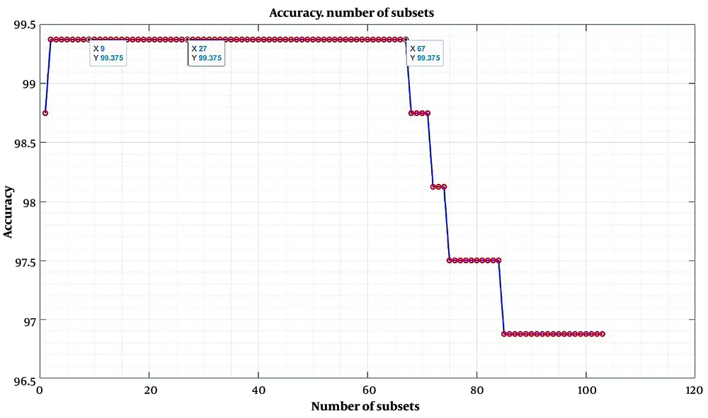
Figure 2.
The plot of the number of feature subsets versus the kNN classifier's accuracy
3.5. Classification Using the k-nearest Neighbor Algorithm (k-NN)
K nearest neighbors is a non-parametric classification method. In k-NN classification, the output is class membership. An object is classified by majority vote among its neighbors, in which the object is assigned to the most popular class among its k nearest neighbors (k is a positive integer, usually small). If k = 1, objects are simply assigned to the single nearest neighbor class. The Euclidean distance is commonly used to find the distance between k nearest neighbors, according to Equation 6 (21).
x, y = Two points in Euclidean k-space
xi, yi = Euclidean vectors, starting from the initial point
k = k-space
In this study, the dataset was first randomly divided into 60% for training and 40% for validation, and class training and evaluation were performed according to the 9 feature subsets. Based on the highest accuracy, the best value of k for this classification was considered to be 5. Figure 3 shows the plot of the coefficient k as a function of accuracy (20).
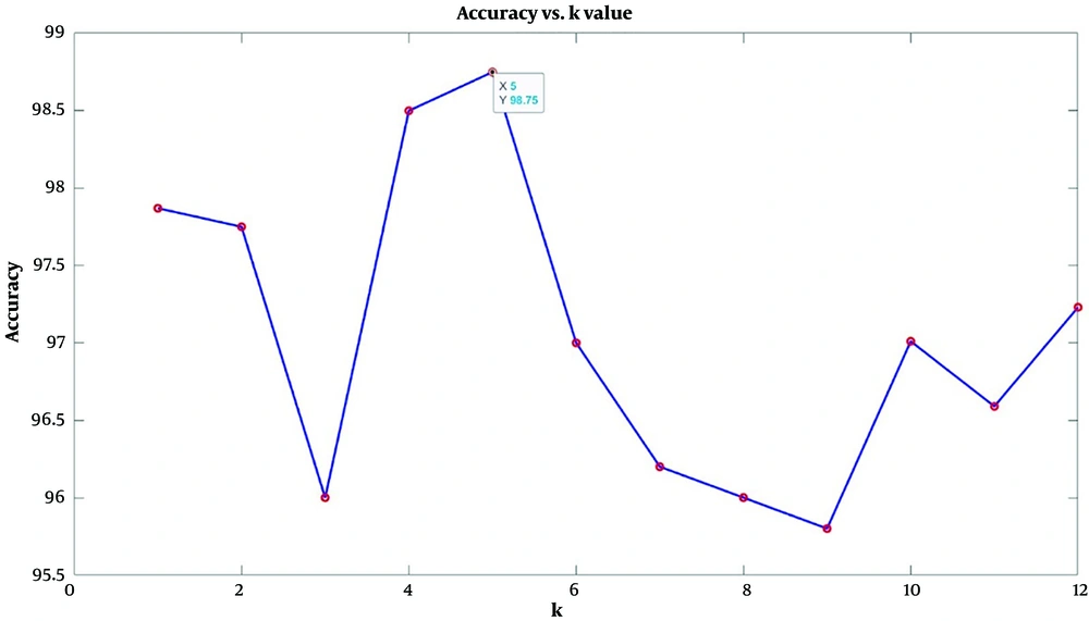
Figure 3.
The plot of the k parameter versus the k-NN classifier's accuracy
4. Results
This study used the dataset of B-mode ultrasound images of the liver. Four hundred cases, including normal and abnormal liver images, were randomly selected in Matlab2022b as the simulation environment. According to the above method, preprocessing and feature extraction were performed. One hundred ten texture features were extracted from these images using the GLCM technique, and only 9 subsets were retained as diagnostic input after dimension reduction.
The texture features were analyzed after processing using a k-NN classifier to obtain the confusion matrix. Performance metrics were used to measure the effectiveness of the design model. These metrics included accuracy, sensitivity, specificity, and mean square error (MSE) for classification problems. The performance of the classifier for the ultrasound dataset is shown in Table 2.
Table 2.
Performance of the k-NN Classifier
| Classifier\Parameters | Accuracy | Sensitivity | Specificity | MSE |
|---|---|---|---|---|
| k-NN classifier | 98.75% | 98.82% | 99.1% | 0.00012 |
5. Discussion
Diagnosis of diseases using medical imaging is very important in medicine. Medical imaging is used to diagnose diseases due to its high accuracy and the possibilities it offers. Considering the limitations of some diagnostic methods, using artificial intelligence seems to be an effective solution for accurately diagnosing diseases.
Hepatocellular carcinoma (HCC) is one of the most dangerous liver diseases. Since it is necessary to diagnose liver diseases based on ultrasound images, developing a computer-aided diagnosis system (CAD) will greatly help physicians make decisions. Therefore, a system to reduce misclassification was proposed in this research.
Although it is impossible to make a direct comparison between each study due to variations in the number of data, databases, feature extraction methods, feature reduction, and classification techniques, it can be concluded, as indicated in Table 1, that image texture feature extraction is highly effective. Furthermore, incorporating highly discriminative features enhances the speed and accuracy of classification and computer-aided diagnosis systems. The procedure for conducting this study is briefly outlined below.
First, 110 texture features, including grey-level co-occurrence matrix (GLCM) features, were extracted from the regions of interest (ROIs). We applied the feature selection procedures to obtain the most relevant features: t-test and SFFS ensemble. Then, we determined the most discriminative feature set. Finally, the k-NN classifier was trained with the features of the training set and tested with the validation set to obtain a reliable result. The final results showed that the proposed methods for a CAD system could provide diagnostic help by distinguishing HCC from normal liver with high accuracy.
This is a preliminary study dealing with two liver stages from the broad spectrum of liver diseases. In future work, the authors would like to incorporate clinical data to observe the characterization of HCC and normal people. In addition, various optimization techniques can improve the accuracy, sensitivity, and specificity of the classification.