1. Background
Nowadays, due to the discharge of different kinds of hazardous materials, especially toxic heavy metals to the surface and groundwater resources through industrial, urban, agricultural and mining effluents and also fuel combustion, evaluation of the groundwater contamination by toxic and essential elements is vital (1-5).
Since heavy metals are not biodegradable they are deposited. They are also characterized by their long persistence or long half-life, assimilated or incorporated in water. They have bioaccumulation potential in the tissues of living organisms, as well. Accordingly heavy metals can cause adverse effects on human health (6, 7). Metals, such as Fe, Cu, Mn, Mo, and Zn are known as an essential elements and play a vital role in biological systems, whereas other elements, such as As, Pb, Cr, Cd, Hg and V are non-essential metals, and due to their toxic characteristics are known as hazardous substances for living organisms (8). Arsenic is a carcinogenic agent to human with no possible beneficial metabolic functions. Exposure to this element can cause some adverse health effects, including anorexia, fever, hair loss, fluid loss, headache, muscle spasms, decrease in the production of blood cells, herpes, nausea, weakness, vomiting, darkening of the skin and, especially liver and kidney failure (9-11). Lead (Pb) as a major global environmental health risk agent can cause serious adverse effects on human health. It has been proved that the consumption of food is the main route for Pb intake into the human body (12, 13). Disruption of the delicate antioxidant balance between the cells and oxidative stress, and also headache, anemia, brain damage, colic, learning disabilities, reduced IQ, hyperactivity, slow growth, and central nervous system disorders are the main adverse health effects of exposure to Pb (14, 15). Zinc (Zn) as an essential element has a functional and structural role in biological systems (16, 17). Exposure to high amounts of Zn can cause nephritis, anuria and also extensive lesions in the kidneys (3, 14, 18).
In the last decade, soft computing models have been successfully applied in solving complex systems in environmental problems. One of the recent methods for training single hidden layer feedforward neural networks (SLFNs) is the extreme learning machine (ELM) suggested by Huang et al. (19) that can significantly enhance the learning process on the networks. Yurtsever et al. (20) applied a fast artificial neural network (ANN) for simulating the removal process of Cd (II) ions by valonia resin. The results indicated that the implemented ANN had better performance compared with the conventional methods. Lima et al. (21) studied the performance of ELM as a reliable method in environmental sciences. Keskin et al. (22) analyzed the application of ANN methods for the estimation of water pollution sources in several stations in Turkey. The results showed the appropriate generalization performance of the ANN model in the prediction of water pollutants. Hossain and Piantanakulchai (23) in 2016 proposed a two-stage approach based on geographic information system (GIS) and classification tree methods to study groundwater resource contamination (heavy metals concentration) risk. The results demonstrated the effectiveness of the two-phase model to predict the degree of accumulation of heavy metals in groundwater resources. Alizamir and Sobhanardakani (24) studied the performance accuracy of an ANN based on the optimization approach of the imperialist competitive algorithm (ANN-ICA) for the prediction of heavy metals contamination in groundwater resources of the Ghahavand Plain. The results of this study indicated that the ANN-ICA model was able to yield high accuracy outputs. Alizamir and Sobhanardakani in 2018 (25) suggested a conjoined methodology based on ANN and particle swarm optimization to simulate heavy metals concentration of Toyserkan Plain. They found that this hybrid model can be effectively utilized for environmental management programs.
To the best of the authors’ knowledge, no study has yet been conducted to estimate heavy metals concentration in Razan Plain using ELM. Therefore, the main aim of this study was to develop an ELM-based model for accurate estimation of heavy metals concentration in groundwater resources of Razan Plain. Besides ELM model, ANN and multivariate adaptive regression spline (MARS) models were also used.
2. Objectives
About 90% of the required water for Razan Plain for domestic and agricultural purposes is provided by groundwater resources. Therefore, this study was conducted to predict toxic and essential elements (As, Pb, and Zn) content in groundwater resources of Razan Plain.
3. Methods
3.1. Study Area
Razan Plain with an aquifer area of about 4810 km2 is located between 49º 20’ eastern longitude and 35º 23’ northern latitude in the northeast of Hamedan, west of Iran. The average annual precipitation of this region is varied from 230 to 300 mm (15).
3.2. Sampling and Sample Preparation
In this descriptive study, a total of 60 groundwater specimens were collected from 20 semi-deep and deep wells along the study area. The specimens were taken in 200 mL polyethylene bottles. Then the collected specimens were filtered through Whatman filter paper No. 42, preserved with 6N of nitric acid (Sigma-Aldrich, Spain) and kept in the refrigerator (4ºC) for further analysis (4). Finally, the contents of As, Pb and Zn were determined using inductively coupled plasma - optical emission spectrometry (ICP-OES; 710-ES, Varian, Australia) in three replicates (4, 7). The statistical parameters (maximum, minimum, mean and standard deviation) of the data are presented in Table 1.
| Element | Min | Max | Mean | SD |
|---|---|---|---|---|
| As | 1.1 | 11.83 | 6.35 | 2.42 |
| Zn | 8.55 | 85.91 | 32.39 | 16.94 |
| Pb | 1.4 | 9.55 | 5.24 | 1.58 |
3.3. Extreme Learning Machine
Huang et al. in 2006 (19) developed a new training algorithm, an ELM for SLFNs to overcome the difficulties of using conventional training schemes. ELM is faster than gradient-based learning implementations and the determination of output weights is based on analytical calculations. Based on the good generalization performance of ELM, this algorithm showed satisfactory accuracy in benchmark problems. ELM using the Moore-Penrose generalized inverse (MPGI) and the minimum norm least-squares solution (MNLS) solves the general linear system Ax = y. The MPGI matrix of A (G) can be defined as:
Also, MNLS for a general linear system can be formulated as:
Where, || || is a norm in the space of Euclidean.
Generally, a standard SLFN with N hidden nodes as well as transfer function g(x) can be described as:
Where, ci and βi are random bias and weight vector for connecting the hidden nodes to the output nodes. H was defined as:
Equation 1 can be written as:
Hβ = Y
By applying the MPGI (H+) of the hidden layer matrix, the weights of outputs can be calculated using MNLS:
In this study, for the ELM model, the sigmoidal activation function was used and the number of hidden nodes was set to 10. This number was obtained using trial and error process.
3.4. Multi-Layer Perceptron Artificial Neural Network
Multi-layer perceptron artificial neural network (MLPANN) is one of the popular soft computing methods, which has been extensively used in different fields of study. MLPANN consists of an input layer, one or more hidden layers and an output layer (26). The neurons are the main processing factor of a neural network. These elements by computing a weighted sum of N input parameters as well as applying transfer functions can yield output values. These models are able to perform complex calculations and yield satisfactory results from experimental data or field observation. In this research, MLPANN was applied for heavy metals concentration prediction in the Razan Plain. In addition, MLPANN with one single layer and Log-Sigmoid as the activation function were also employed for the estimation of heavy metals concentration in Razan Plain. Moreover, the efficient algorithm of Levenburg-Marquardt used to accelerate the convergence process of the network (27).
3.5. Adaptive Regression Spline
Friedman in 1991 (28) introduced an MARS as a nonlinear and nonparametric regression approach. This method applies high dimensional parameters for mapping a group of inputs to the output variables (29). At the first step, MARS, by dividing predictors into the subgroups, generated a basic function for each subgroup. The basic functions handle data properties of the one or several input parameters and they make the relation between independent and dependent parameters (28). It can be noted that the basic functions are placed between two points, beginning and end, which are called knote (30). The MARS model can be expressed as:
Where, Y is the output parameter, P and B are the number of inputs and basic functions, respectively.
3.6. Evaluation Criteria
In this study, three reliable statistical indicators were applied to investigate performance evaluation using soft computing models for the estimation of heavy metals concentration in Razan Plain.
1) Coefficient of determination (R2) (Equation 8)
2) Pearson correlation coefficient (r) (Equation 9)
3) Root mean square error (RMSE) (Equation 10)
Where, n is the total number of data and Pi and Oi are the simulated heavy metals concentration values by the developed methods and measured values, respectively.
4. Results
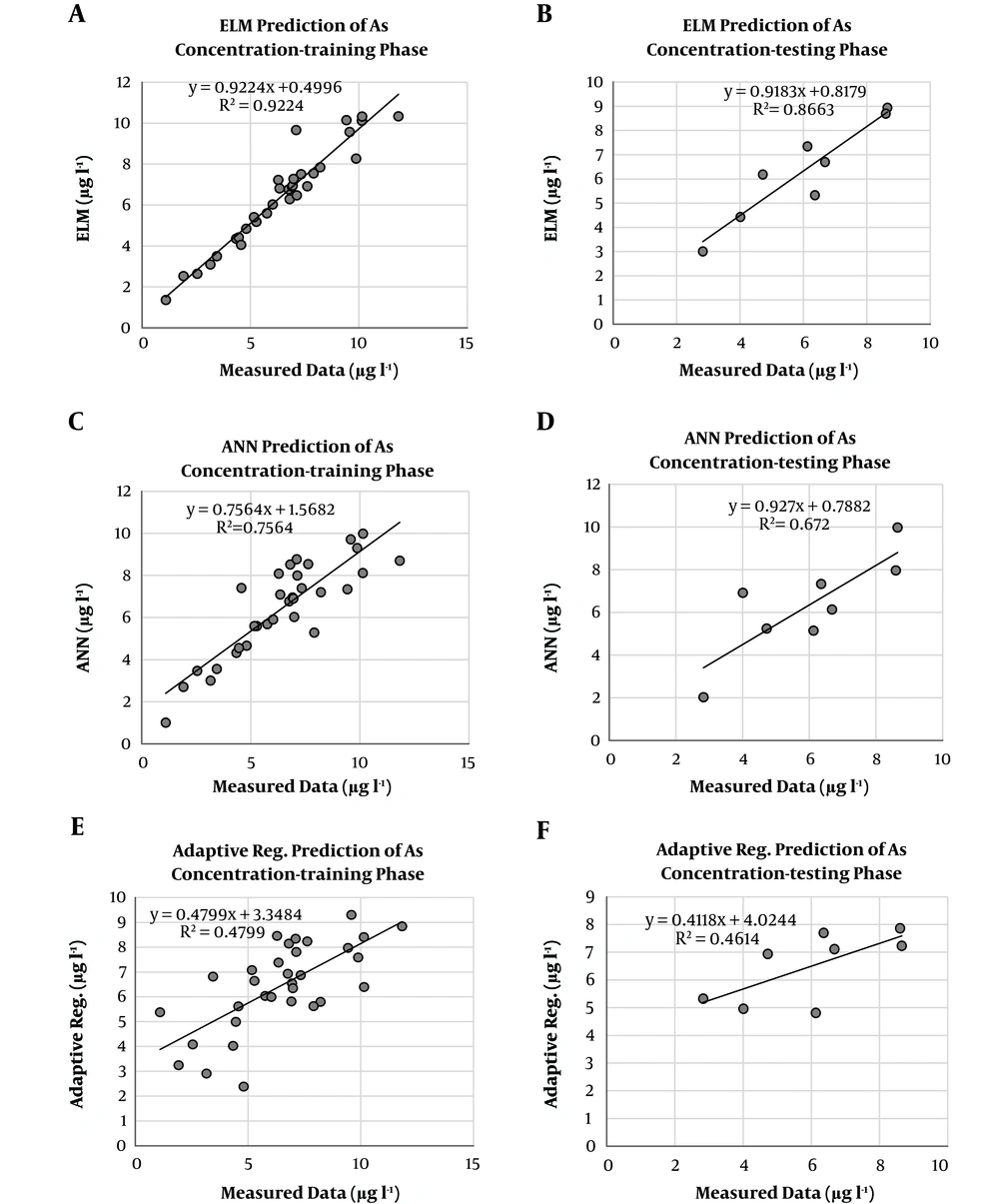
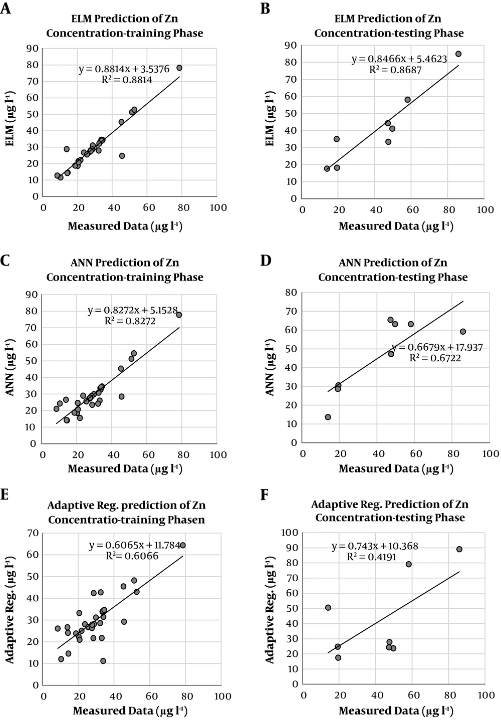
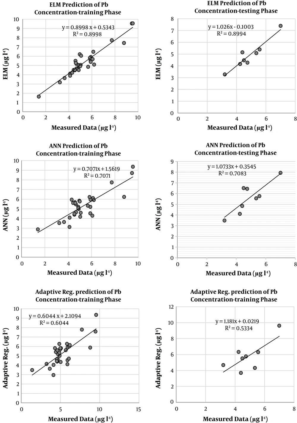
ELM models were developed for predicting heavy metals concentration in Razan Plain. Previous data of Zn, As and Pb were used as input parameters to the ELM models. As mentioned before, for comparing the results of the developed models, three reliable statistical indicators were used using RMSE, correlation coefficient and coefficient of determination to obtain the best model. ELM, ANN and MARS models were compared for the training and testing phases in Table 2. Various numbers on hidden nodes were tried for ELM and ANN models to find the optimum ELM and ANN structures. For example, in the ANN model, 500 iterations, 10 hidden nodes, and sigmoid transfer function for the hidden and output nodes led to the optimum results. Based on Tables 2-4, it is clear that the ELM model performed better than the ANN and adaptive regression models in the testing phases to estimate three heavy metals concentration. The lowest RMSE and highest R2 and r values were gained by the ELM models. The concentration estimates of the ELM, ANN and MARS models in the training and testing phases are illustrated in Figures 1-3 for As, Zn, and Pb concentration. According to these figures, the superiority of the ELM model over ANN and MARS models is quite evident. For the ELM, ANN and MARS implementations, program codes were written in MATLAB (R2014b) environment.
| Heavy Metal Concentration | Methods | Training | Testing | ||||
|---|---|---|---|---|---|---|---|
| RMSE | r | R2 | RMSE | r | R2 | ||
| As | ELM | 0.693 | 0.960 | 0.922 | 0.788 | 0.930 | 0.866 |
| ANN | 1.229 | 0.869 | 0.756 | 1.310 | 0.819 | 0.672 | |
| Adaptive regression spline | 1.796 | 0.692 | 0.479 | 1.512 | 0.679 | 0.461 | |
| Heavy Metal Concentration | Methods | Training | Testing | ||||
|---|---|---|---|---|---|---|---|
| RMSE | r | R2 | RMSE | r | R2 | ||
| Zn | ELM | 4.729 | 0.938 | 0.881 | 8.305 | 0.931 | 0.868 |
| ANN | 5.707 | 0.909 | 0.827 | 13.516 | 0.819 | 0.672 | |
| Adaptive regression spline | 8.612 | 0.778 | 0.606 | 20.680 | 0.647 | 0.419 | |
| Heavy Metal Concentration | Methods | Training | Testing | ||||
|---|---|---|---|---|---|---|---|
| RMSE | r | R2 | RMSE | r | R2 | ||
| Pb | ELM | 0.524 | 0.948 | 0.899 | 0.362 | 0.948 | 0.899 |
| ANN | 0.896 | 0.840 | 0.707 | 1.017 | 0.841 | 0.708 | |
| Adaptive regression spline | 1.042 | 0.777 | 0.604 | 1.482 | 0.730 | 0.533 | |
5. Discussion
To investigate the applicability of the developed ELMs, after obtaining the optimal architecture and parameters of each model, they were trained to find the best biases and weights to yield the lowest error values. Comparisons of the results showed that the ELM model with the sigmoid activation function yielded the best results in both training and testing phases (Table 2) for the studied heavy metals concentration. Figure 1A and B shows the predicted and observed concentration of the As in both training and testing phases using the ELM model. As displayed in this figure, it is quite evident that during the training phase, the ELM model predicted the concentration of As better than the testing phase. The estimates of ANN and MARS are shown in Figure 1C - F. As can be seen in Table 2, the prediction of the ELM model with the RMSE, r, and R2 of 0.788, 0.93, and 0.866 was more favorable than ANN and MARS with the RMSE, r, and R2 of 1.31, 0.819, and 0.672 and 1.512, 0.679, and 0.461, respectively.
For Zn concentration, the results of the ELM, ANN and MARS are given in Table 3. The highest RMSE and the lowest r and R2 values were obtained by MARS, whereas the highest R2 value was achieved by ELM model. It can be said that the ELM model was more effective in predicting Zn concentration. The estimates of the ELM model for both training and testing phases are demonstrated in Figure 2A. Also, Figure 2B and C shows the results obtained by ANN and adaptive regression models. The figures emphasize the better performance of the ELM model compared with the ANN and adaptive regression models. According to Table 3, the ELM model estimated the Zn concentration in testing phase with R2 = 0.868, RMSE = 8.305 and r = 0.931, the ANN model predicted with R2 = 0.819, RMSE = 13.516 and r = 0.819, and the MARS model forecasted with R2 = 0.419, RMSE = 20.68 and r = 0.647. In general, the ELM model seems to be more adequate than the ANN and adaptive regression models for the prediction of Zn concentration.
The results of ELM, ANN and adaptive regression spline to estimate Pb concentration in the training and testing phases are provided in Table 4. The highest r and R2 and the lowest RMSE values were obtained by ELM for the estimation of Pb concentration. Among the ELM, ANN, and adaptive regression spline, the MARS yielded the worst results. Figure 3 demonstrates the results of three machine learning models in both training and testing phases. The ELM model significantly outperforms the ANN and MARS models. The ELM predicted Pb concentration with R2 = 0.899, RMSE = 0.362 and r = 0.948 and improved the prediction accuracy by 64% and 75%, compared with the ANN and adaptive regression models, respectively.
Yadav et al. (31) have reported a good generalization performance of the ELM approach in surface water management. Heddam and Kisi (32), have stated that an ELM model is suited for the prediction of water quality parameters using the observed data. Also, Alizamir et al. (33) have applied the ELM approach for efficient modeling water level fluctuations using hydro-climatic parameters. In another study, Kisi and Alizamir in 2018 (34) have reported that the ELM model can yield satisfactory results compared with the conventional soft computing models. Based on the results, it is clear that the ELM model can be utilized as a robust artificial intelligence approach to estimate the concentration of various heavy metals in Razan Plain. The findings of this study suggested the ELM model as a reliable alternative to investigate environmental variables, such as groundwater resource contaminations. Using the suggested ELM model in other environmental problems is suggested to establish sustainable policies to facilitate the protection of the environment.
5.1. Conclusions
This study investigated the effectiveness of ELM approach to estimate heavy metals concentration in Razan Plain using the collected data. ELM approach was compared with ANN and MARS models using RMSE, correlation coefficient, and coefficient of determination. Comparison of the results showed that the effectiveness of ELM model compared with the ANN and MARS models. By applying the ELM models, the RMSEs were reduced in comparison with ANN and MARS models. Totally, it was found that the concentration of heavy metals in groundwater resources could be successfully predicted by ELM using the available data in the Razan Plain.


