1. Background
In functional magnetic resonance imaging (fMRI) studies, the physical parameters of the brain change in response to a given task. Regional increase in blood flow rate is the parameter, which could be activated with a specific stimulation. Cerebrovascular reactivity (CVR) is the change of cerebral blood flow in response to a vasoactive stimulus (1, 2)
Determining activated brain areas due to different activities is one of the most common targets in fMRI data analysis, which could be carried out by hemodynamic response function (HRF) evaluation (1, 3-6).
Neurovascular connections can be non-invasively studied based on the HRF information. Thus, HRF modeling plays an important role in fMRI data analysis and evaluation of the cerebrovascular diseases (4, 7, 8). The HR functions reflect changes of cerebral blood flow (CBF) in response to neural activity (1, 3, 4). This function is different between subjects and has a significant variation between brain regions. Therefore, correct HRF modeling could enhance the accuracy of fMRI studies (1). Intensity, onset latency, and duration of the underlying brain metabolic activity were evaluated based on HRF shape characteristics (including height, delay, and duration) (5). Hemodynamic response function parameters, including time to peak (T) and height (H) provide information about brain area activation, and full-width at half-max (W) of a stimulated HRF determines the time of activity (5).
The fMRI task design has a considerable effect on the efficiency and detection power of the study. Previous studies indicated that event-related designs have high estimation efficiency with poor detection power. However, good detection power at the cost of low estimation efficiency is achieved using block designs (9). Block designs are mostly used in BOLD fMRI studies. Therefore, selection of the best model to estimate HR functions in block design studies could have a critical role in patient data analysis.
2. Objectives
In this study, five models including gamma (GAM) (10), inverse logistic (IL) (11), the canonical HRF plus its temporal and dispersion derivatives (DD), canonical HRF plus its temporal derivative (TD) (12, 13), and finite impulse response (FIR) models (14, 15) were evaluated to estimate HR function of a simulated dataset. Models with higher accuracy were used to determine HRF parameters of patient data.
3. Methods
3.1. Hemodynamic Response Function Models
The relationship between blood oxygenation level dependent (BOLD) response and stimulus is presented using the Equation 1:
Where y (t) is the signal at time t and is the convolution between the hemodynamic response (h(t)) and stimulus (s(t)) functions. In these studies, a fixed canonical shape is assumed for h(t) (10).
The HRF was estimated based on five models, including gamma (GAM), inverse logistic (IL), canonical HRF plus its temporal and DD, canonical HRF plus its TD, and finite impulse response (FIR) models. The Lindquist approach was used to determine the HRF parameters (5).
3.2. HRF Model Selection
Akaike’s information criterion (AIC), Schwarz’ Bayesian (SBC), and mean square error (MSE) criteria were used to select the best HRF estimation model. The AIC, SBC, and MSE indices are described in Equations 2 - 4
Where n and p are sample size and number of parameters, respectively. The model with the least amounts of AIC, SBC, and MSE had a better performance for HRF estimations.
3.3. Data Simulation
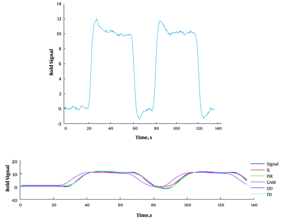
The simulated BOLD signal was produced based on real data. Changes have been regularly quantified in terms of commencement and period of neural activity. The stimulus function was convoluted with SPM’s canonical HRF to produce the simulated signal. It was assumed that repetition time (TR) and duration of stimulation were 3 and 120 seconds, respectively. The onset stimuli were presented in 60 and 240 seconds. The dataset consisted of the BOLD signal plus white noise. Furthermore, a random interpersonal variance with a standard deviation equal to one-third of interpersonal variance was added to each time series. On the simulation study, five models were fitted on the simulated BOLD signal. The simulation studies were repeated one hundred times. The HRF features, including T, H, and W indices, were extracted for each fitting model.
3.4. FMRI Data Acquisition
The fMRI data were acquired in a 3 Tesla Siemens (Munich, Germany) MAGNETOM TIM Trio scanner using a 12-channel Matrix head coil (Siemens Medical Systems, Erlangen, Germany). Functional MR images with BOLD contrast were acquired using an echo-planar imaging (EPI) sequence. The applied scanning parameters were: TR = 3 seconds, TE = 30 msec, flip angle = 90°, matrix size = 64 × 64, and voxel size = 3 × 3 × 3 mm3.
3.5. FMRI Task Design
For fMR imaging in block design, CO2 gas was administered using a face-mask under physiological monitoring. The FMRI data were registered by administration of CO2 for 120 seconds with 60-second rest intervals. The HRF in the cerebral areas with higher blood supply was determined based on changes in blood CO2 level.
3.6. Data Processing
The FMRI data were processed using the MATLAB software (version 8.6, The MathWorks TM, Natick, Massachusetts, United States). The simulation procedures were repeated 100 times and the best HRF estimation models were selected. Then, these models were implemented on the patient data. The fMRI data analysis was performed using the SPM 12 MATLAB toolbox (Wellcome Trust Center for Neuroimaging).
3.7. Patient Data
Three patients with brain tumors (two males and one female; mean age, 28.33 years; age range, 21 to 34 years) were imaged. The study was approved by the local committee for medical research ethics. Informed consent was obtained from the patients prior to the study.
4. Results
4.1. Data Simulation
The simulated signal is depicted in Figure 1A. For time series estimation, the efficacies of the models were evaluated. The standard and estimated time series by five models are shown in Figure 1B. As it could be seen from the Figure 1, the estimated signals by IL, FIR, and TD models are in acceptable consistency with the standard time series.
A, the simulated signal in block-design method, TR = 3 seconds, onset = 60 and 240 seconds, duration = 120 seconds, block length = 420 seconds. B, The estimated signals by five mentioned models. The standard time series is also depicted. Abbreviations: DD, the canonical HRF plus its temporal and dispersion derivatives, FIR, finite impulse response; GAM, gamma; IL, inverse logistic; TD, the canonical HRF plus its temporal derivative models.
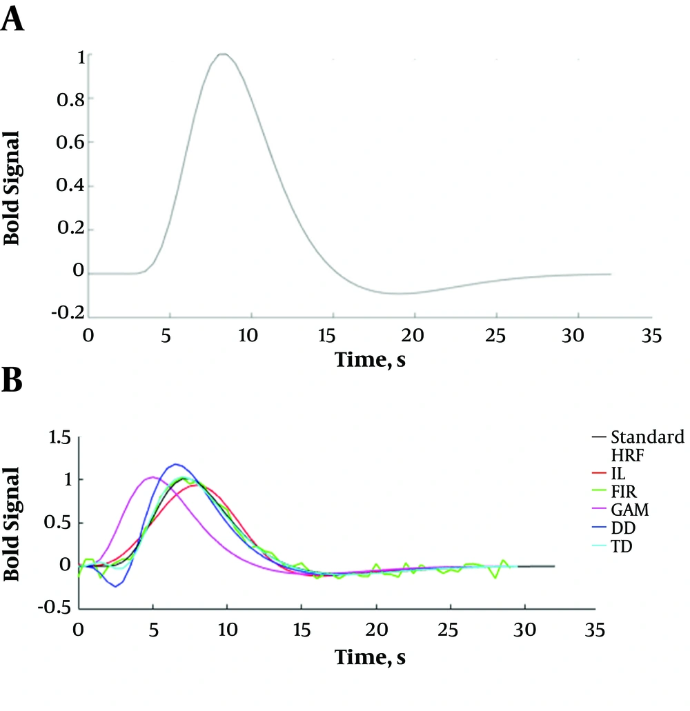
For determining the best HRF estimation model, an HRF was produced as the standard function and it was estimated by five HRF estimation models.
The standard HRF is illustrated in Figure 2A. Figure 2B shows the estimated HRFs by five models. In Figure 2, the standard HRF is also depicted. The estimated HRFs by IL, FIR, and TD models were almost equal to the standard HRF.
A, illustration of the standard HRF. B, The standard and estimated HRFs by five models. Abbreviations: DD, the canonical HRF plus its temporal and dispersion derivatives, FIR, finite impulse response; GAM, gamma; IL, inverse logistic; TD, the canonical HRF plus its temporal derivative models.
A scatter plot was used to evaluate the model efficiency for signal estimation. For the best model with acceptable efficiency to estimate the simulated signal, spots would be more closely located around the bisector of the first quadrant. The results of IL, FIR, and TD models are almost placed around the bisector of the first quadrant. The simulation procedures were repeated 100 times and the average values of H, T, and W parameters were registered. The characteristics of the estimated HRFs (including H, T, and W) are listed in Table 1. For each HRF estimation model, MSE, AIC, and SBC indices were also listed in the Table 1. The standard values for H, T, and W indices were 1, 7.5, and 5.5, respectively. From the Table 1 and the visual evaluation, it could be concluded that IL, FIR, and TD models present better HRF estimation than the other models.
| Standard | TD | DD | GAM | FIR | IL | |
|---|---|---|---|---|---|---|
| Time to peak | 7.5 | 7.5 | 7 | 5.5 | 7 | 8.3 |
| Height | 1 | 1.008 | 1.178 | 0.7912 | 0.9992 | 0.8912 |
| Width | 5.5 | 5.5 | 5 | 5.5 | 6 | 5.8 |
| MSE | - | 0.052 | 0.105 | 0.146 | .055 | 0.068 |
| AIC | - | -1235.1 | -883.5 | -175.8 | -1206.4 | -1091.5 |
| SBC | - | -1223.9 | -871.5 | -165.7 | -1194.9 | -1049.2 |
The Characteristics of the Estimated HRFs by Five Modelsa
4.2. Patient Data Analysis
The efficiency magnitudes of five HRF estimation models were evaluated based on a simulated time series. The best HRF estimation models were selected to analyze the patient data. Three patients with brain tumors were imaged in block-design fMRI paradigms. The selected models were used to estimate HR functions of the patient data.
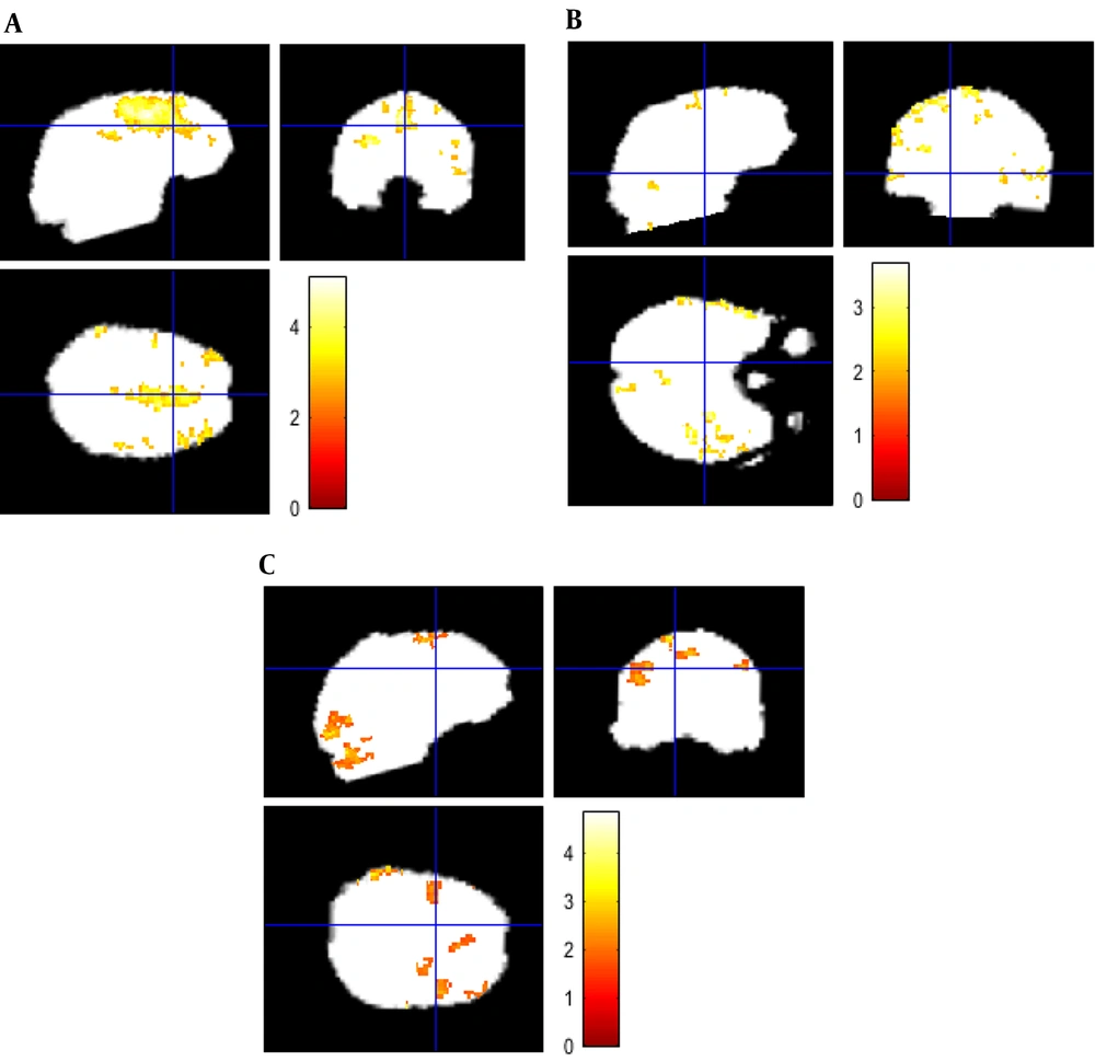
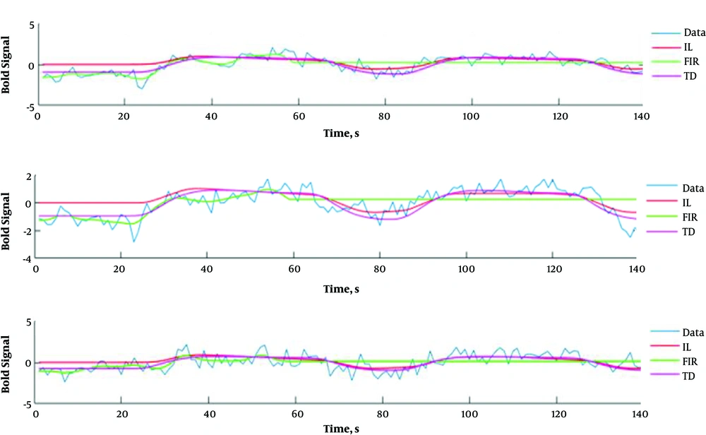
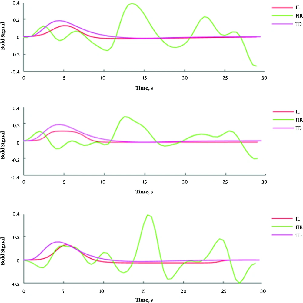
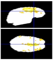
Figure 3 shows cerebral regions with higher blood supply in three patients with brain tumors. The subjects’ data were analyzed with P value = 0.001, voxel threshold = 20, onset stimulus = 60 and 240, and duration of stimulation = 120 seconds. For the patients, the areas with higher blood supply were placed at the frontal, temporal, and occipital lobes, respectively. Figure 4 shows the estimated signals using models at the cerebral area with higher blood supply. The estimated HRFs by IL, FIR, and TD models are illustrated in Figure 5.
The block-design fMRI signals of the patients and the results of the fitted IL, FIR, and TD models on the signal. For each patient, the block-design fMRI signal and the related fitted models were depicted in separate sub figures. Abbreviations: FIR, finite impulse response; IL, inverse logistic; TD, the canonical HRF plus its temporal derivative models.
The average values of H, T, and W indices at the regions of interest (ROIs) are listed in Tables 2 - 4, respectively. The MSE, AIC, and SBC indices are also listed in Tables 2 - 4 for each model.
| IL Model | FIR Model | TD Model | |
|---|---|---|---|
| Height | 0.076577 | 0.071911 | 0.121912 |
| Time to peak | 4.184738 | 12.79348 | 4.195652 |
| Width | 3.934783 | 2.413043 | 3.043478 |
| MSE | 0.143363 | 0.23641 | 0.135698 |
| AIC | -266.9885 | -196.4844 | -273.88888 |
| SBC | -258.1636 | -187.6595 | -265.0638 |
The characteristics of HRF for a 32-year-old woman with brain tumor
| IL Model | FIR Model | TD Model | |
|---|---|---|---|
| Height | 0.089164 | 0.099497 | 0.139391 |
| Time to peak | 4.21001 | 14.23241 | 4.265332 |
| Width | 3.334783 | 3.251252 | 3.122598 |
| MSE | 0.091099 | 0.186892 | 0.088393 |
| AIC | -330.416 | -229.8149 | -334.6386 |
| SBC | -325.8137 | -220.9900 | -321.5914 |
The characteristics of HRF for a 34-year-old man with brain tumor
| IL Model | FIR Model | TD Model | |
|---|---|---|---|
| Height | 0.093541 | 0.075221 | 0.116532 |
| Time to peak | 4.205297 | 12.442018 | 4.152324 |
| Width | 3.652218 | 3.102328 | 3.25138 |
| MSE | 0.121870 | 0.220289 | 0.108532 |
| AIC | -289.6759 | -206.7976 | -305.9025 |
| SBC | -280.8510 | -197.9726 | -297.0776 |
The characteristics of HRF for a 21-year-old man with brain tumor
5. Discussion
The mentioned models were fitted on the simulated signal in block-design studies. Figure 2A shows that all of the models, except gamma, can fairly estimate simulated BOLD signal. The standard and estimated HRFs by each model are shown in Figure 2B. Figure 2 visually shows that TD, FIR, and IL models estimate the simulated HRF. The estimated HRF by the DD model has a higher height than the simulated HRF and the estimated HRF using gamma model has a different time to peak than the simulated HRF. Also, the estimated HRF using the IL model has a different time to peak and height yet these differences could be ignored. For simulation studies, which were repeated 100 times, average magnitudes of T, W, and H indices were registered. For the canonical HRF plus its temporal derivative model, the characteristics of the estimated HRF were closer to the standard HRF. The MSE, AIC, and SBC indices were ignorable for TD, FIR, and IL models, which indicates that these models could accurately estimate HRF in a block-design fMRI study. From the model selection criteria and the characteristics of the estimated HRFs, it could be concluded that TD is the best model for HRF estimation.
In Lindquist et al.’s studies, seven models, including canonical HRF, canonical HRF plus TD, canonical plus TD and DD, FIR, sFIR, two-parameter gamma distribution, and total three IL models were evaluated to estimate HRF. The patients wore a heat arm band scaled in event-related method (warm, mild painful, fairly painful and pain threshold) and then they were imaged. The results showed that the IL model estimates HRF better than TD and sFIR models. The TD model yields the weakest estimation of HRF (5, 11).
In this study three selected models were evaluated on real data. Figure 5 shows the signals of cerebral areas with higher blood supply and the results of the fitting models. As it could be seen from the Figure 5, the models have been acceptably fitted on the given signal, and TD model has the best fitting trend line. A square region of interest (3 × 3 pixels in size) was extracted to evaluate the cerebral areas with higher blood supply and their averages of T, W, and H magnitudes. The MSE, AIC, and SBC indices were smaller for the TD model. Unlike Lindquist et al.’s study, the TD model has a better HRF estimation for block-design fMRI data. In Lindquist et al.’s study, the IL model provides a better HRF estimation for event-related data (5). In Shan et al.’s study HR function (in block-design method) was modeled using five models, including the canonical HRF used in SPM8, canonical HRF, the sum of two and three gamma functions, and the sum of three inverse logit functions used by Lindquist et al. It was found that in the event-related method, four IL models had a higher efficiency for HRF estimation. However, the results of real data (in block-design method) showed that two-gamma with six parameters had the best HRF estimation (16).
5.1. Conclusions
In the present study, HRF modeling of the cerebral area with higher blood supply was investigated. For a simulated dataset, HRF modeling was evaluated using five models. Based on the results, TD, FIR, and IL models were selected for HRF modeling in a block-design method. These models were used to analyze the block-design fMRI data for patients with brain tumors. The results showed that the TD model yields better HRF estimation to evaluate the changes in human cerebral blood flow. These models could be helpful to investigate the change of signal intensity under CVR conditions, non-invasively.
.jpg)
