A New Model for Epidemic Spreading with a Focus on COVID-19

Babak Jamshidi; Mansour  Rezaei; Khansa Rezaei

doi:10.5812/jhealthscope.102837

https://doi.org/10.5812/jhealthscope.102837

A New Model for Epidemic Spreading with a Focus on COVID-19

authors:

Babak Jamshidi ¹ , avatar Mansour Rezaei ^{2
, *} , Khansa Rezaei ³

1 Department of Biostatistics, Kermanshah University of Medical Sciences, Kermanshah, Iran

2 Social Development and Health Promotion Research Center, Kermanshah University of Medical Sciences, Kermanshah, Iran

3 Educational Development Center, Kermanshah University of Medical Sciences, Kermanshah, Iran

Health Scope: Vol.9, issue 3; e102837

published online: July 18, 2020

article type: Methods Article

received: March 18, 2020

revised: May 16, 2020

accepted: June 9, 2020

how to cite: Jamshidi B, Rezaei M , Rezaei K. A New Model for Epidemic Spreading with a Focus on COVID-19. Health Scope. 2020;9(3):e102837. https://doi.org/10.5812/jhealthscope.102837.

Abstract

Background:

It is extremely useful to construct mathematical models to forecast and control real phenomena. One of the common applied statistical models to represent the data involving with time is the time series modeling. A novel time series model to represent the propagation of an epidemic infection in a population is presented. The model deals with addressing the cumulative number of confirmed cases.

Methods:

Our model is the generalization of statistical exponential growth models and can describe different stages of the outbreak of a communicable disease. Applying the mentioned procedure leads to models CVJR1 (3.2, 1.44, 3, 13) for modeling the sequence of COVID-19 from January 13 to March 5. All computations and 200 simulations were done in MatLab 8.6.

Results:

For comparing candidates through fitting the dataset for six pairs of (

\hat{l}

and

\hat{a}

), we used the minimum criterion square of residuals. We present the average and 90% upper and lower bounds of the predictions made by our models for three periods. Applying the mentioned procedure led to having models with parameters (3.2, 1.44, 3, 13) for modeling the course of COVID-19 from January 13 to March 5.

Conclusions:

The presented model can cover the epidemic behaviors related to social networks. Our model can be adjusted to worldwide modeling for modeling a phenomenon spreading in different populations simultaneously.

Keywords

Epidemic COVID-19 SARS Model Spreading Estimation

1. Background

Contagious diseases are a major cause of human suffering in terms of both morbidity and mortality. The essence of these diseases is their transmission, which is the main subject of studies addressing the issue in various science branches. One of the approaches to query in this subject is the mathematical one. Mathematical models are caricatures of real systems that aim to capture the fundamental mechanisms of some processes to explain observations or predict outcomes (1). The idea of formulating the transmission and spread of infectious diseases in mathematical language is relatively old. Its history backs to 1760 when Bernoulli (2) published an article to describe the effects of smallpox variolation on life expectancy using mathematical life table analysis (3). The modern mathematical modeling, initiated in 1920, has evolved over the years in an impressive body of works, whose culmination can be found in Anderson et al. (4).

For modeling a communicable disease, there are two main approaches founded on the time as the basis and independent variable: the macro-dynamic and micro-dynamic approaches. The classic model that ignores the structure of the population and views the population as a generality is of the former group, and the network models that focus on the interactions of individuals of the population and stress the importance of configuration of the population in details are of the latter group (1).

From another point of view, there are two main approaches to dealing with an epidemic model: deterministic and stochastic. The network models are the most known in the stochastic class. There are some examples of this class in the literature (5-8). The differential equation models (ODE and PDE), including the KM model (9) and statistical exponential growth models, are two known families of deterministic models. Time series models can be categorized as stochastic macro-dynamic models. In addition, to some extent, time series modeling in epidemiological applications is restricted to ARIMA models (10-12). Finally, it is worth saying that there are some novel methods in this area, including artificial intelligence methods and two-part time series (13, 14).

To the extent of our knowledge, the models introduced so far are restricted to modeling some periods of the outbreak of the disease. This drawback motivated us to present a new model. We presented a novel model, which is more convenient than graphical models, and it is competent enough to cover epidemiological spreading and epidemic behaviors related to social networks like the pattern of the number of users of Facebook, the number of confirmed cases of SARS in China, and the number of COVID-19 cases worldwide.

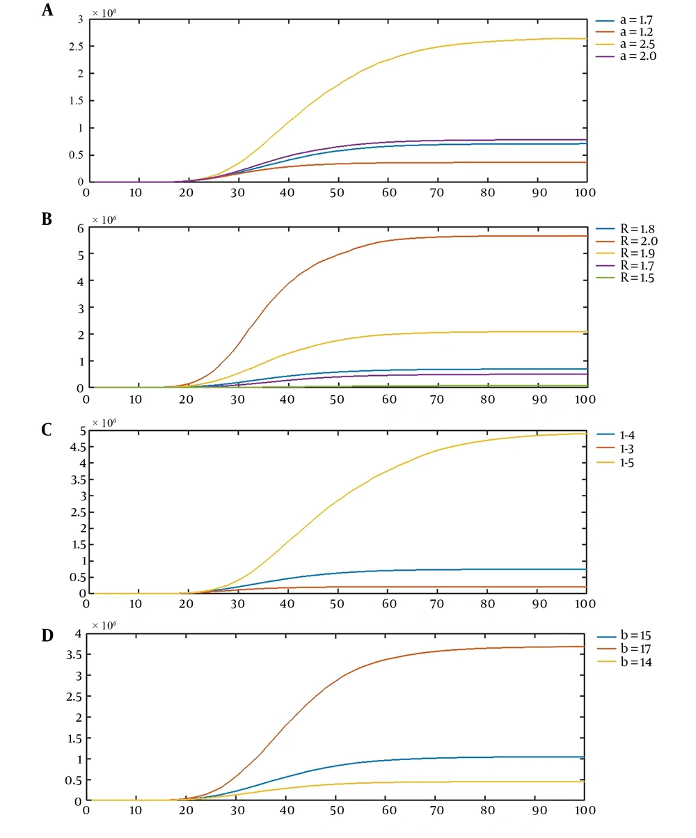
Our stochastic model is flexible enough to cover different stages of a communicable disease from the initial stage with an intense growth through the stage of identification and then implementation of prevention and control measures to its retreatment and discovery of treatment. This flexibility is well illustrated by plots that show the effect of changing each of the parameters of the model on its behavior (Figure 1).

Figure 1.

A, The first scenario for the effect of the values of parameters on realizations of the model, the average curves of CVJR (a, 1.8, 4, 15), for a = 1.2, 1.7, 2.0, 2.5; B, the second scenario for the effect of the values of parameters on the realizations of the model, the average curves of CVJR1 (1.7, R, 4, 15), for R = 1.5, 1.7, 1.8, 1.9, 2.0; C, the third scenario for the effect of the values of parameters on the realizations of the model, the average curves of CVJR1 (1.7, 1.8, l, 15), for l = 3, 4, 5; D, the fourth scenario for the effect of the values of parameters on the realizations of the model, the average curves of CVJR1 (1.7, 1.8, 4, b); for b = 14, 15, 17.

The presumption of utmost importance about our time series model is that in the beginning, the disease spreads exponentially and as time goes by, the rate of transition (λ), the reproductive number (R₀), or the rate of the growth of the number of infected individuals (R in our model) tends to fall. This presumption is a common fact in all known epidemic models. Britton et al. (15) mention this point as a challenge regarding the modeling of the outbreak of communicable diseases. The mentioned behavior is observed in connection with the time series of several infected cases of SARS 2003, the timeline of the number of people using social media platforms and the internet, worldwide or nationwide, and the time series of MERS outbreak in South Korea and Saudi Arabia between 2013 and 2020. Also, this assumption is met by the time series of the positive cases of COVID-19. For example, in 10 days from January 22, the number reached from 580 to 11,950 (over 20 times or more than 1900% growth), while this number over 10 days from February 22 increased from 78,651 to 88,590 (about 13%). Based on this reality, we classify the behavior of infection spreading into three stages:

Stage 1. The initiation of the disease (This stage in the following formulation is considered as step 1).

Stage 2. The beginning of the awareness, precaution, and control measures (This stage is step 2 in the following formulation).

Stage 3. The phase of the retreatment of the disease (This stage includes steps 3, 4, 5, and so on in the formulation).

To the best of our knowledge, mathematical epidemic models mainly address stage 1, and in the most advanced cases, deal with stage 2.

In comparison with graphical models, our model is explicitly time-oriented. Also, it is more flexible and more convenient. One of the main problems in applying random network models is the entrance of the infection to new populations. For example, COVID-19 has arrived in over 140 countries up to now. Therefore, to model it graphically, it is required to have 140 different graphs connected (or at least, five different graphs for China, South Korea, Iran, Italy, and Japan). It is noticeable that our model is more flexible and more informative than non-graphical models. In addition, the present model gives information on the stage of intensity and the process of change in the stages of intensity.

2. Methods

2.1. Presumptions of the Model

The model is based on the following presumptions:

The number of susceptible individuals is proportional to the rate of growth (the relative increment).

The rate of growth is fixed in the first days of the propagation; therefore, the cumulative number of confirmed cases follows an exponential trend.

The trend of time series of growth rate is decreasing. At first, it faces a significant sudden decrease, and then it falls gradually.

Several successively lower growth rates lead to lower growth rates in the following days (due to increasing the steps or stages).

Based on the presumptions, the model is not suitable to represent the propagation of epidemics in which after some severe limitations (quarantine, staying home, social distancing, etc.), the condition of the population comes back to the previous status. To model this sort of epidemics, we need to update the model by changing the step of the model.

2.2. Mathematical Definition of the Model

We present a model to cover all the three stages; CVJR1 (a, R, l, b). This model is a stochastic process (time series model) with four parameters:

a: Representation of the decreasing probability of the rate of spreading corresponding to different items in a specified step.

We assume that the probability of acute outbreaks decreases exponentially, and conversely, the probability of mild and gradual increments increases.

R: The rate of the growth in the initial days (the first b days) of the spreading.

It is worth noting that one of our model’s presumptions is that the number of infected cases rises exponentially in the first b days. Thereafter, R, which depends on parameters a and l, falls. The role of R in our model is analogous to the role of R₀ and λ in macro-dynamic and micro-dynamic models, respectively.

l: The number of days of absence of the more intense epidemiological behavior of the disease that ensures us that the level of the spreading of the infection has decreased by one step (The criterion for specifying the retreat of the disease from a more intense step to a less intense step).

b: The number of the first days that the infection faces no resistance or control.

Our model is formulated as follows:

I. The Initial Condition:

S t e p_{1} = S t e p_{2} = \dots = S t e p_{b} = 1

and

S t e p_{b + 1} = 2

I t e m_{1} = 1

U (1) = U (2) = \dots = U (b - 1) = 0

X_{1} = 1

II. The Evolution Law:

S t e p_{(t + 1)} = S t e p_{t} + \prod_{j = 1}^{l} U (t - j)

t = b + 1, b + 2, \dots

I t e m_{(t + 1)} = 1 + I t e m_{t} (1 - S t e p_{t + 1} + S t e p t_{t})

t = b, b + 1, \dots

U (t + 1) ~ B e r n o u l i (e^{- a \times I t e m_{(t + 1)}})

t = b, b + 1, b + 2, \dots

X_{t + 1} = X_{t} (1 - \frac{1}{R^{{S t e p}_{(t + 1)} + U (t + 1) - 1}} + \frac{1}{R^{{S t e p}_{(t + 1)} + U (t + 1) - 2}})

t = 2, 3, 4, \dots .

Therefore, we can classify this model as an autoregressive multivariate time series.

X_t: The number of infected individuals up to time t.

Step_t: Determining the phase of the outbreak of the disease.

As mentioned before, by this indexing, steps 3, 4, and so on are considered together as the step of retreat or stage 3 of the infection (in this case, COVID-19).

Item_t: The item of the disease in a special step.

Here, the variable item is more detailed and more partial than the variable step. By variable item, we are equipped with a tool to meet the decreasing trend of the rate of transition, reproductive number, or growth rate during a specified step.

U(t + 1): A function whose input is the variable item to determine the intensity of the spread of the disease during a time unit (in this model, the time unit is taken as one day, and it can be replaced with one month, one week, one hour, and so on).

The computations and simulations of the paper were done in MatLab 8.6. Throughout the paper, each curve is obtained through 200 simulations. In all figures, the X and Y axes represent the days and the number of confirmed cases, respectively.

Four scenarios illustrate the flexibility of our model and its capacity to cover a great variety of real datasets (Figure 1A-D).

Increasing a leads to descending the probability of acute growth periods; therefore, the plot becomes smooth earlier and the range of the axis Y decreases. The lower the parameter a is, the more the intensity of the outbreak of the disease is. As R increases, the growth rate of the number of infected cases goes upper. Therefore, the height of the plot rises, and the slope of the plot increases. According to this model, by declining l, the condition for the change in phases (retreat of the process) gets harder. Therefore, the plot tends to increase by a higher acceleration. Finally, b is the length of the most intense spread. Then, the more the value of b is, the more the increase in the number of cases will be. To illustrate the novel method, let (a, R, l, b) = (0.9, 2.5, 4, 11). Our model suggests the first stage of the spreading of infection (Table 1).

Table 1.

The Realization of the First Stage of the Outbreak of the Infection According to Our Model (CVJR1)

Day	1	2	3	4	5	6	7	8	9	10	11
Number of cases	R⁰	R¹	R²	R³	R⁴	R⁵	R⁶	R⁷	R⁸	R⁹	R¹⁰
Rounded number	1	2	6	16	39	98	244	610	1526	3815	9537

The continuation of spreading (stage 2) is sometimes like its previous phase and sometimes like its current phase (Table 2).

Table 2.

A Realization of the Second Stage of the Outbreak of the Infection According to Our Model (CVJR1)

Item	1	2	3	4	5	6
Current number	9537^a	23842	38147	61035	97656	156249
Previous phase^b	3815	9537^a	15259^a	24414^a	39063^a	62500
U	0	1	1	1	1
Intensity	More	less	less	less	less

^aThe figures determine the numbers that multiplying them by (1 - R) is equal to the growth of the process.

^bPrevious phase is not $X_{i - 1}$ . It is equal to $X_{i} / R$ .

Since the parameter l is taken equal to 4, four consecutive 1s lead to a movement from step 2 to step 3 (generally, from step n to step n + 1). Accordingly, the results show the continuation of the process during stage 3 (Table 3). The evolution in step n is similar to the second step, but in this step, 1 and 0 correspond to n - 1 and n - 2 steps before, respectively.

Table 3.

A Realization of the Third Stage of the Outbreak of the Infection According to Our Model (CVJR1)

Item	1	2	3	4	5	6	7
Current number	156249	193749	240249	297909	476655	591052	732904
Previous phase	62500	77500	96100	119164^a	190662	236421	…
Two phases ago	25000^a	31000^a	38440^a	47665	76264^a	94568^a	…
Run	1	2	3	0	1	2	…
U	1	1	1	0	1	1	…
Intensity	less	less	less	more	less	less	…

^aThe figures indicate the numbers that multiplying them by (1 - R) is equal to the growth of the process.

It is noticeable that the variable run presents the number of consecutive 1s (less acute outbreak). It is observed that happening zero for the variable U or increasing the steps makes this variable equal to zero immediately. Accordingly, the following sequence is obtained as a realization of our model:

1, 2, 6, 16, 39, 98, 244, 610, 1526, 3815, 9537, 23842, 38147, 61035, 97656, 156249, 193749, 240249, 297909, 476655, 591052, 732904, ...

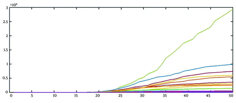
By repeating this procedure, we can obtain 15 realizations (Figure 2).

Figure 2.

Some realizations of the present model with parameters (0.9, 2.5, 4, 11)

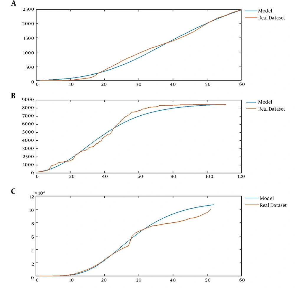
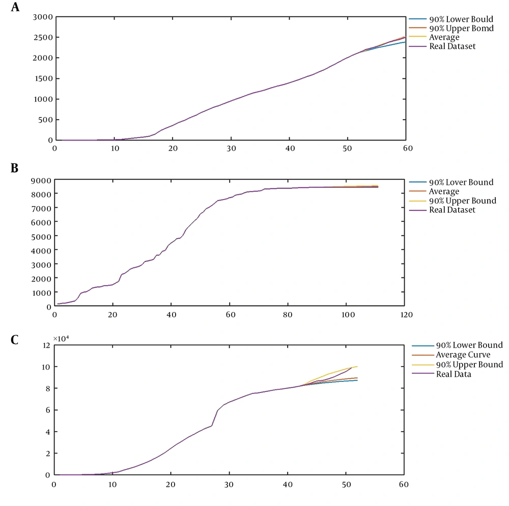
Now, we address the flexibility of the introduced model that enables the model to represent a wide range of epidemic data. The validity of the model is assessed in two ways: the ability to model past observations and the validity of predictions of the model. The former is illustrated by Figure 3, while Figure 4 implies the latter ability of the model. The average curve of the realizations of our model could fit some known datasets, such as the pattern of the number of users of Facebook (16), the number of confirmed cases of SARS in China (17), and the number of infected cases of COVID-19 worldwide (18) (Figure 3A-C).

Figure 3.

A, The mean curve of CVJR1 (0.75, 1.35, 3, 1) for modeling the sequence of Facebook users from 2014 to 2019; B, the mean curve of CVJR1 (0.6, 1.23, 2, 2) for modeling the time series of confirmed cases of SARS in China from March 17 to June 17; C, the mean curve of CVJR1 (3.2, 1.44, 3, 13) for modeling the procedure of COVID-19 from January 13 to March 5.

Figure 4.

A, Modeling the first time series using our model (CVJR1), the mean curve, 90% upper bound, and 90% lower bound with parameters (0.75, 1.35, 3, 1) for prediction of the sequence of Facebook users in 2018 - 2019 (eight units); B, modeling the second time series using our model (CVJR1), the mean curve, 90% upper bound, and 90% lower bound with parameters (0.6, 1.23, 2, 2) for prediction of time series of confirmed cases of SARS in China, from May 18 to June 17 (30 units); C, modeling the third time-series using our model (CVJR1), the mean curve, 90% upper bound, and 90% lower bound with parameters (3.2, 1.44, 3, 13) for prediction of the procedure of COVID-19 from February 25 to March 5 (10 units).

3. Results

3.1. Estimation of the Parameters

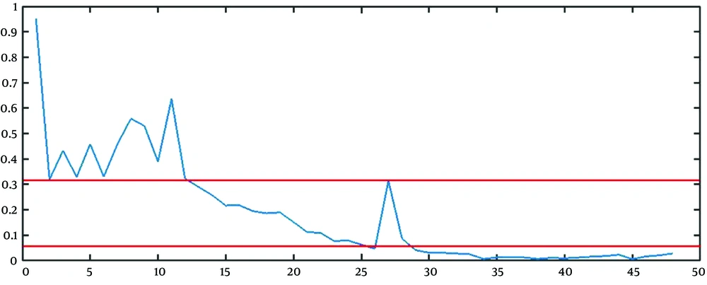
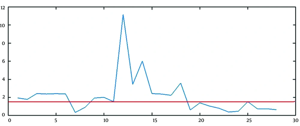
The best approach to find the estimation of parameters is to combine the mathematical and graphical methods. The main informative observations to estimate are x_t (observed time series), Dr_t = r_t - 1 = (x_t+1 - x_t)/ x_t, and DDr_t,m= Dr_t/Dr_t+m as depicted in Figure 3C, 5, and 6, respectively.

Figure 5.

The sequence of Dr_t from t = 1 to t = 48; two red lines represent two bounds for the irreversible falls (t = 13 and t = 28)

Figure 6.

The sequence of DDr_t,m from t = 16 to t = 43 and m = 6 (ignoring the first days of spreading); the red lines represent the geometric mean of the data depicted

The graphical method is simple and fast, but somehow immature. The points that the rate falls irreversibly (without recursion to the previous range) can be considered as the breakpoint, the finish point of a step, and the start point of another step. For example, in Figure 5, t = 13, and t = 28 are two change points. It is worth saying that except for the first breakpoint, the number of steps shifted from or shifted to, is probably unknown in other breakpoints. For example, it is not clear that the lower line in Figure 5 determines the breakpoint of step 2 to 3, step 3 to 4, or step 4 to 5.

To estimate R and b, we used the geometric mean of the rate of growth of the points belonging to stage 1 (from t = 1 to t = 13 in Figure 5) and the number of points of stage 1 (13 in Figure 5) as $\hat{R}$ and $\hat{b}$ , respectively. It is noticeable that the parameter b is better to be estimated clinically as the length of the non-symptomatic period of the disease. Moreover, since our model is the generalization of the statistical exponential growth models, the methods applied to find the exponential rate of growth in that model can be helpful.

The next step is to estimate the parameter l. For finding $\hat{l}$ , steps 2 and above can be helpful. Regarding the model, we have the following equation:

$D_{R t} = R - 1$ , for t belonging to step 1.

$D R_{t} = (R^{2 - i} - R^{1 - i})$ or $(R^{3 - i} - R^{2 - i})$ , for t belonging to steps i > 1.

Based on this calculation, it is reasonable to expect that mean of (Dr_t / Dr_t+m= $\hat{R}$ ) for t in step i and t + m in step i + 1

Accordingly, we clustered the data into some groups, each of which includes m time points. Therefore, the estimation of m can be the integer value for m that leads to clustering with a geometric mean of (Dr_t / Dr_t+m) close to $\hat{R}$ . Figure 6 is the representation of the sequence of Dr_t / Dr_t+m for t = 16, 17, 18, …, 43, and $\hat{m}$ = 6. The red line is the geometric mean of ratios, approximately 1.6. If we set $\hat{m}$ greater than 6, the range of the fraction widens upward and the geometric mean of the ratios grows. On the other hand, taking $\hat{m}$ less than 6 can result in the shrinkage of the figure and fall in the geometric mean.

For the reasons above, we can set $\hat{m}$ = 6 as the estimation of the mean of the length of a step. Correspondingly, the length of a run of the less intense level of spreading in a step (as the requisite for going to the upper step) must be equal to or less than 6. Therefore, $\hat{l}$ = 1, $\hat{l}$ = 2, $\hat{l}$ = 3, $\hat{l}$ = 4, $\hat{l}$ = 5, and $\hat{l}$ = 6 are our alternatives. For each of these alternatives, we calculated the best-fit estimator for the parameter a to meet the condition that the length of a step is expected to be 6.

In our model, setting p = exp(-a), Table 4 is obtained as the representative of changing the probability of spreading intensity for different items of each step.

Table 4.

Evolution of Probability of Intensity of Growth for the Items of Each Step

Item	1	2	3	…	L - 1	l	L + 1	…
Probability of more intense	p	p²	p³	…	p^l-1	p^l	p^{l + 1}	…
Probability of less intense	1 - p	1 - p²	1 - p³	…	1 - p^{1 - 1}	1 - p^l	1 - p^{l + 1}	…

For the positive integer random variables like the length of a stage (M), expectations can be calculated with the equation.

E (X) = \sum_{i = 1}^{\infty} P (X \geq i)

Since $M \geq l$ ,

E (M) = \sum_{i = 1}^{\infty} P (M \geq i)

To calculate this summation, it is convenient to consider the probability of complements;

E (M) = \sum_{i = 1}^{\infty} (1 - P (M < i))

To solve this equation, we require the following recursive equation;

$P (M < i) = 0$ for $i < l$

P (M < i) = \sum_{j = 0}^{i - l - 1} P (M \geq (j - 1)) p^{j} (1 - p^{j + 1}) (1 - p^{j + 2}) \dots (1 - p^{j + l})

for $i \geq l$

Therefore, for obtaining the most suitable estimation for the parameter a, we need to find the root of the following equation numerically;

\sum_{i = 1}^{\infty} (1 - \sum_{j = 0}^{i - l - 1} P (M \geq (j - 1)) {\hat{p}}^{j} (1 - {\hat{p}}^{j + 1}) (1 - {\hat{p}}^{j + 2}) \dots (1 - {\hat{p}}^{j + l})) - \hat{m} = 0

Now, we can estimate the parameter a by using

\hat{a} = - l o g (\hat{p})

The last step is to compare our candidates through fitting the dataset (x_t). Our candidates are six pairs of ( $\hat{l}$ and â). Our criterion in this item is the minimum square of residuals.

Applying the mentioned procedure leads to having models with parameters (0.75, 1.35, 3, 1), (0.6, 1.23, 2, 2), and (3.2, 1.44, 3, 13) for modeling the sequence of Facebook users from 2014 to 2019, the time series of confirmed cases of SARS in China from March 17 to June 17, and the course of COVID-19 from January 13 to March 5, respectively (Figures 3A-C and Figures 4A-C). In Figure 4, we present the average, 90% upper bound, and 90% lower bound of the predictions made by these models in the periods from 2018 to 2019 (eight units), May 18 to June 17 (30 units), and February 25 to March 5 (10 units).

4. Discussion

The novel time series model in the present paper can represent epidemic behaviors, including social and infectious spreading. This model is based on some presumptions. Therefore, it does not work well when the decreasing trend of the rate of growth is absent because it is the main presumption of the model. Also, since the information on the initial days is of utmost importance for this model, one of the challenges in this model is its modification to get qualified to model datasets that lack information on the first days. For example, in connection with COVID-19, if we model the spreading of the disease after March 1, information on the first days is absent. To overcome this challenge, we were forced to gather data before the WHO reports. The rationale behind this is that spreading exponentially in the first days is one of the assumptions of our model, too.

The model is not suitable to represent the propagation of epidemics in which after some severe limitations (quarantine, staying home, social distancing, etc.), the condition of the population comes back to the previous status. To model this sort of epidemics, we need to update the model by changing the steps of the model.

It is noticeable that the model is dynamic, and similar to other time series models, the estimations need to be updated because our data are limited. Generally, if we have more information, we can obtain booster models and more accurate estimations. In addition, the implementation of strict prevention and control measures, the intense spread of the disease, or the emergence of new epicenters of spread such as in South Korea and Iran necessitate new estimations for each model, particularly ours. It is worth saying that to overcome this challenge, we applied a mechanism to return the process to the previous step when a new epicenter of spread is found.

Finally, we suggest that the function of this model be evaluated by comparing it with other families of time series and artificial intelligence methods.

4.1. Conclusions

We can promote the accuracy of modeling the disease by considering it locally or by country. It is trivial that at present, the stage of the outbreak in Iran is quite different from its stage in other countries such as China and South Korea. In modeling infections worldwide, it is very helpful to apply a mechanism to decrease the steps of the process by one level when a new epicenter of spread is found.

Footnotes

Authors' Contribution: BJ did idea, computation, simulation, and the first draft. MR did adjusting the model, final draft, and discussion. KR did editing and literature survey.
Conflict of Interests: All authors declare that they do not have any conflict of interest.
Funding/Support: None.

References

1.
Jamshidi B, Alavi SMR, Parham GA. The distribution of the number of the infected individuals in a stochastic SIR model on regular rooted trees. Commun Statistics-Simulation Comput. 2019:1-18. https://doi.org/10.1080/03610918.2019.1584299.
2.
Bernoulli D. Essai d'une nouvelle analyse de la mortalité causée par la petite vérole, et des avantages de l'inoculation pour la prévenir. Histoire de l'Acad Roy Sci (Paris) avec Mem. 1760:1-45.
3.
Dietz K, Heesterbeek JA. Bernoulli was ahead of modern epidemiology. Nature. 2000;408(6812):513-4. [PubMed ID: 11117719]. https://doi.org/10.1038/35046270.
4.
Anderson RM, Anderson B, May RM. Infectious diseases of humans: Dynamics and control. UK: Oxford university press; 1992.
5.
Greenwood M. On the statistical measure of infectiousness. J Hyg (Lond). 1931;31(3):336-51. [PubMed ID: 20475096]. [PubMed Central ID: PMC2170634]. https://doi.org/10.1017/s002217240001086x.
6.
Bartlett MS. Some evolutionary stochastic processes. J Royal Statistic Soc. 1949;11(2):211-29. https://doi.org/10.1111/j.2517-6161.1949.tb00031.x.
7.
Klovdahl AS. Social networks and the spread of infectious diseases: The AIDS example. Soc Sci Med. 1985;21(11):1203-16. [PubMed ID: 3006260]. https://doi.org/10.1016/0277-9536(85)90269-2.
8.
May RM, Anderson RM. Transmission dynamics of HIV infection. Nature. 1987;326(6109):137-42. [PubMed ID: 3821890]. https://doi.org/10.1038/326137a0.
9.
Kermack WO, McKendrick AG. A contribution to the mathematical theory of epidemics. Proceedings of the royal society of london. Series A, Containing papers of a mathematical and physical character. 1927;115(772):700-21.
10.
Perone G. An ARIMA model to forecast the spread of COVID-2019 epidemic in Italy. SSRN Electron J. 2020. https://doi.org/10.2139/ssrn.3564865.
11.
Tabataba FS, Chakraborty P, Ramakrishnan N, Venkatramanan S, Chen J, Lewis B, et al. A framework for evaluating epidemic forecasts. BMC Infect Dis. 2017;17(1):345. [PubMed ID: 28506278]. [PubMed Central ID: PMC5433189]. https://doi.org/10.1186/s12879-017-2365-1.
12.
Li Q, Guo NN, Han ZY, Zhang YB, Qi SX, Xu YG, et al. Application of an autoregressive integrated moving average model for predicting the incidence of hemorrhagic fever with renal syndrome. Am J Trop Med Hyg. 2012;87(2):364-70. [PubMed ID: 22855772]. [PubMed Central ID: PMC3414578]. https://doi.org/10.4269/ajtmh.2012.11-0472.
13.
Ribeiro M, da Silva RG, Mariani VC, Coelho LDS. Short-term forecasting COVID-19 cumulative confirmed cases: Perspectives for Brazil. Chaos Solitons Fractals. 2020;135:109853. [PubMed ID: 32501370]. [PubMed Central ID: PMC7252162]. https://doi.org/10.1016/j.chaos.2020.109853.
14.
Jamshidi B, Rezaei M, Najafi F, Sheikhi A. The prediction of COVID-19 spread in Iran from 15 March to 15 April 2020. Iran Red Crescent Med J. 2020;22(5). https://doi.org/10.5812/ircmj.102822.
15.
Britton T, House T, Lloyd AL, Mollison D, Riley S, Trapman P. Five challenges for stochastic epidemic models involving global transmission. Epidemics. 2015;10:54-7. [PubMed ID: 25843384]. [PubMed Central ID: PMC4996665]. https://doi.org/10.1016/j.epidem.2014.05.002.
16.
The statistics of Facebook users. 2016. Available from: https://sproutsocial.com/insights/social-media-statistics/.
17.
WHO. Severe acute respiratory syndrome 2003 (SARS) situation reports. 2003. Available from: https://www.who.int/csr/sars/country/en/.
18.
WHO. Coronavirus disease 2019 (COVID-19) situation report: 1 to 40. 2020, [cited 2020 Feb 26]. Available from: https://www.who.int/docs/default-source/coronaviruse/situation-reports/20200225-sitrep-36-COVID-19.pdf?Sfvrsn=2791b4e0_2.

comments