1. Background
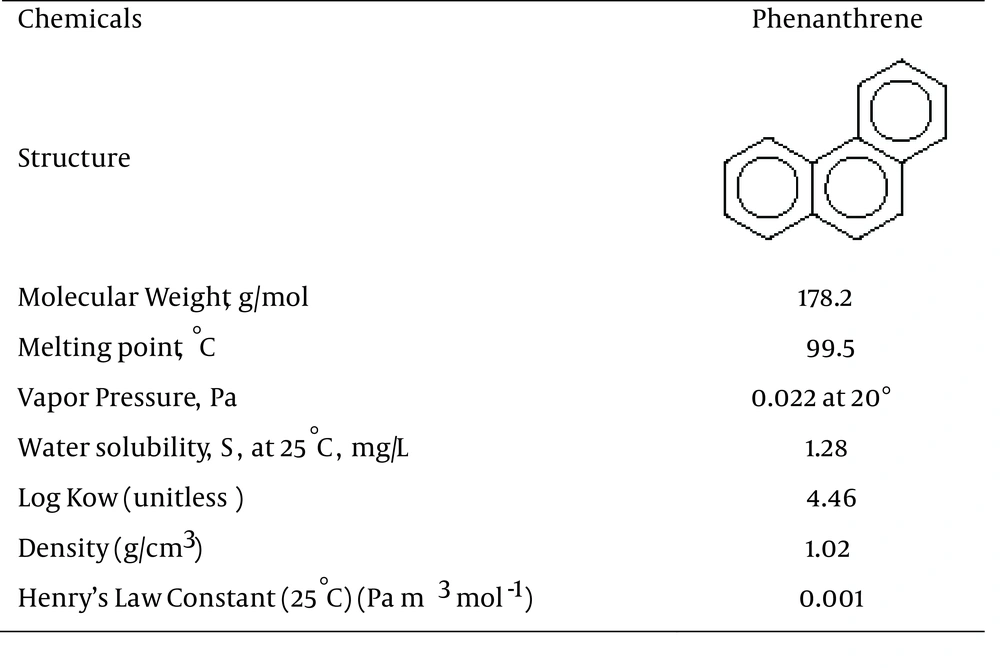
Polycyclic aromatic hydrocarbons (PAHs) are abundant and important environmental non-ionic pollutants. These organic compounds, which are extracted from emissions of anthropogenic sources, annually comprise their largest part worldwide (1). Synthetically, PAHs are formed during anthropogenic activities such as incomplete burning or pyrolysis of carbon-containing materials like coal, wood, oil products and garbage in air-deficient environments (2), which like other similar contaminants, can be found globally in different amounts in soils (3, 4) and can be identified in a variety of waters and wastewaters. They rarely dissolve in water, but have solubility in organic solvents and are highly lipophilic (5). Phenanthrene, a polycyclic aromatic hydrocarbon (PAH), is an important class of organic pollutants, mainly because of its wide distribution in the environment and its carcinogenic and mutagenic properties (6, 7). The chemical structure and attributes of the phenanthrene are shown in Figure 1 (8).
Organic pollutants are of concern because they have toxic effects on living organisms including human. These toxic effects can be either acute or chronic and include disruption of the endocrine, reproductive and immune systems, neurobehavioral disorders, and carcinogenicity (8).
Depending on PAH type and exposure mode, exposure to these pollutants has contributed to an increasing risk of cancer development in different tissues including bladder, lung, stomach, skin and scrotum (9). As an organic pollutant, phenanthrene is also toxic and can enter human body through ingestion, breathing, or skin sorption. It is known as a human skin photosensitizer and mild allergen, and under specialized conditions, it is mutagenic to human microbial system (10).
Existence of PAHs in the environment and especially in soil causes a serious risk to human health over each food chain. To describe fate and behavior of organic contaminants, numerous environmental scholars have confirmed and used two parameters: (i) the soil sorption coefficient (Kd) and (ii) the soil organic carbon sorption coefficient (Koc). These parameters show the strength of contaminants’ sorption to obtain surfaces at the water/solid interface; thus, it can demonstrate the environmental mobility and persistence (11). The higher their values, the more strongly the pollutants are absorbed to the interface, and consequently, they would be less moveable (12).
Several models such as constant partition coefficient, practical parametric Kd model, and empirical equations have been suggested to estimate Kd values. General equations predicting Kd , mostly derived empirically from statistical analysis, possess a linear or nonlinear polynomial framework; though, their accuracy is not so satisfactory (13).
Due to variances in the experimental conditions, chemical-based techniques for predicting Koc involve measurement errors. Even when these variations are accepted statistically, property measurements are costly and laborious (14). The methods applied to estimate Koc act in accordance with the statistical relationships with other attributes such as octanol/water partition coefficient (Kow), water solubility (S), molecular descriptors (e.g. first-order molecular connectivity index, and bioconcentration factors (BCF)) (15, 16). In fact, the relationships, suggested in the literature, expressed in a log-log form, were obtained by regression: Log (Koc) = a Log (S, Kow, or BCF) + b (a and b are constants). Chemical property estimation programs like AUTOCHEM estimate Koc from Kow using the ‘Log (Koc) = -0.55 Log (Kow) + 1.377’ equation. The CHEMEST computer program, which estimates chemical properties, allows the user to estimate Koc using equations similar to those used by AUTOCHEM (17). Karickhoff et al. (18) studied Kow and Koc for a series of polycyclic aromatics and chlorinated hydrocarbons including phenanthrene and obtained a correlation coefficient of 0.98 between them. Evaluating the detailed absorptive behavior of four PAH compounds with various chemical and structural characteristics, Means et al. (19) reported an extremely significant correlation between Koc and Kow, both in log form (R2 = 0.98). Karickhoff (20) developed equations for estimating Koc from S and Kow. The correlation coefficients for linear and logarithmic forms between Koc and Kow were 0.994 and 0.997, respectively. Investigating the relationship between the topological indices and the sorption coefficient (Koc), Tao and Lu (21) analyzed the molecular connectivity indices and polarity correction factors based on 543 chemicals, employing a stepwise regression for their effect on a linear model. Subsequently, they developed a linear model using three indices of molecular connectivity along with a set of polarity correction factors, whose R2 values were greater than 0.86. Toul et al. (22) obtained an empirical relationship between Koc and Kow values, which is applicable for a variety of values with both parameters and for a wide scale of pollutants/absorbents. Based on various topological molecular descriptors, Mishra et al. (23) also built several quantitative structure-activity relationship (QSAR) models to estimate the Koc of the replaced anilines and phenols, and reported that a tetra-parametric model was optimal for re- modeling such compounds. However, the complexity of soil and environmental behavior led to studies that attempted to present more simplified models with lower and easier-to-obtain required data.
Artificial Neural Networks (ANNs), like other elastic and systematic methods that are more appropriate than the empirical models, were used for adapting the nonlinear relationships and complicated interactions (i.e. hidden relationships between input variables). Recently, ANNs have become common tools employed by scholars to predict the amount of contamination and concentration of various effluents and chemicals available in drinking water, wastewater, and groundwater. ANNs are mostly applied to diverse issues reflecting successful results (24, 25). Likewise, several scholars have proved the applicability of ANN to adsorption systems (26-28). Gao et al. (14) used linear regression and ANN to predict Koc from Kow and S. Diaconu et al. (27) used ANN for estimating the amount of phosphate pollutant adsorption and its adsorption rate to soil, and confirmed the capability of ANN. Similarly, Snidgha (28) applied an optimization approach to create a neural network with three layers to predict the efficacy of removing phenol pollutant from aqueous solution, using peat soil as an adsorbent.
To the best of our knowledge, unfortunately, there is no work regarding phenanthrene sorption coefficients (Kd and Koc) modeling using soil organic matter (SOM) as input data, especially with the aid of artificial neural networks. Therefore, the aim of the current study was to investigate the accuracy of ANN models with minimum required data for estimating Kd and Koc and for modeling the pollutant (phenanthrene).
1.1. Artificial Neural Networks Model
As a processing inspired tool, an ANN is similar to biological nervous systems in processing information and includes a variety of highly interconnected processing elements (neurons) working together for problem solving. Being able to extract meaningful relationships from complex or vague data, ANNs are used to detect complicated formats and trends, which can be too challenging for humans (27). Like natural networks, some neurons receive problem data (input layer neurons) in these models, whereas some other ones (hidden layer neurons) process them and another group (output layer neurons) present answer (29). Therefore, each neural network has its own input and output layers whose neuron amount is determined by the given problem, and the decision designer (decision maker) will set the hidden layer (the number of its neurons). In this layer, i.e. network training, the procedure of determining connection weights for neurons with purpose of finding the set of weights between the neurons can determine the minimum number of errors processed. To allocate the connection weights, the gathered data of the examples of the given issue were used. Then, a computer program was used to determine the relative weights and to represent the problem behavior using the mentioned information. This process was corresponding with the network fitting to the training data (27). Next, the values allocated to the input layer were multiplied by the weights of their own cells and of the next cells, and then, they were transferred to the following layer. Finally, all the inputs were summed in the next layer and the results were derived from its activity task, resulting in the cell’s output. The obtained rates of the latter layer included the responses offered for the problem, which would be the main answers after comparing with the observed values, if the calculation error was acceptable (30). The usual algorithm for training networks is back propagation (BP). In BP, which is a supervised learning method, error values are calculated after each learning cycle and then the weight correction signals are distributed in the network. One of the most important parts used for determining the optimal structure of ANN is determining the number of neurons in hidden layer and achieving the lowest error, which is obtained by trial and error (31). Compared to other methods, an advantage of the ANN model is that it does not need previous information about relations between inputs and outputs. In addition, it is less sensitive to error in input data. In other words, by using the minimum measured parameters, this model is able to predict target variables variation precisely (32).
1.2. Artificial Neural Networks Description
To design and train the ANNs, a series of input and output including organic content and phenanthrene sorption coefficients, respectively, was necessary.
Due to the limited number of data and to obtain more reliable results, a cross-validation was used for selecting the best performing models which provides a means for building different training/testing splits guaranteeing that each data point is present at least once in the testing set. The whole phase is simple: (i) split the data into equal-sized groups. (ii) for I = 1 to n, select group i as the testing set and all other (n-1) groups as the training set. (iii) Train the model on the training set and measure it on the testing set. This iteration is called a fold. In general practice, setting n = 10 or 10-fold cross-validation is accepted, as it provides a very accurate estimate of the generalization error of the model (33).
As far as there were 32 input samples in this study, an eight-fold cross-validation was used. To perform this procedure, the input data were divided into eight equally-(or nearly equal) sized parts (folds). Then, eight series of iteration of training and validation were conducted. During each step, a various segment of the data was used for validation and the other folds were used for training. Next, the trained models were used to predict the validity of data. Therefore, a network was once built and assessed with a new set of data. Due to performing a reliable test on a smaller set of data and a number of computational attempts, this procedure seems superior to the simpler trained-and-tested process, and results in eight networks.
The normalization of inputs is crucial for preventing any decrease in speed and correctness of network, as well as making data values equal (34). After normalizing the data by Equation 1, the mean of the data series was 0.5 (35).

Where xn is the normalized value, x is the actual value, x-bar xm is the mean value, xmin is the minimum value, and xmax denotes the maximum value of parameter.
For modeling with ANN, a multilayer perceptron (MLP) network was used with MATLAB 7.6 software. Changing weights among different layers, which is called training process, was repeated till the least differentiation between observed and predicted data is obtained. In this process, the learning rule was Marquardt-Levenberg using the sigmoid and hyperbolic tangent (Tansig) functions (31). Finally, the trial-and-error method was employed to calculate the number of neurons per hidden layer.
2. Objectives
Reviewing the literature, there was no such work that could predict phenanthrene sorption coefficients (Kd and Koc) using soil organic matter as input data employing ANNs; hence, this technique was used in this study to calculate the sorption coefficient of the mentioned contaminant. The current research was an attempt to delve into the ability of ANN models in forecasting Kd and Koc varieties regarding various values of soil organic carbon, and introducing the most accurate model with the minimum required inputs. Eliminating the need for laborious and costly laboratory experiments, the resulted model would be suitable for estimating the sorption coefficient of phenanthrene in soils similar to the one used in the present study.
3. Materials and Methods
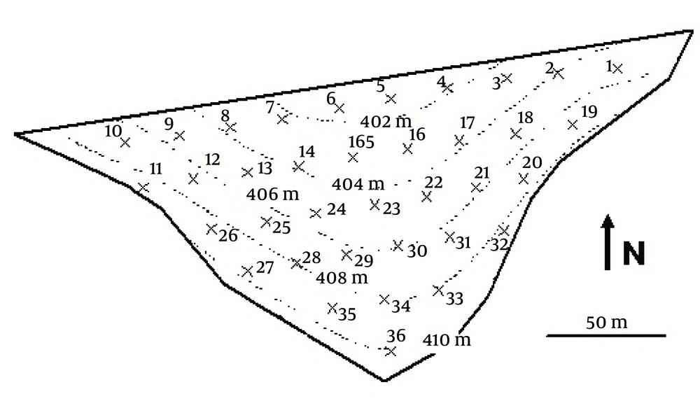
As shown in Figure 2, the required data of the present study were taken from the experiments carried out on soils from a paddock under pasture at Flaxley agriculture centre, mount lofty ranges, South Australia. The soils comprised a set of ferric and eutrophic red chromosols on the upper to mid-slopes and mottled eutrophic yellow chromosols on the lower slopes (36).
Sorption experiments were carried out using a batch equilibration technique at 25°C. To minimize variation in ionic strength and to avoid dispersion, 0.01 M CaCl2 was used as a background solution. Moreover, 200 mg L-1 HgCl2 was used as a microbial growth inhibitor (37). At the end of the equilibration period, suspensions were centrifuged at 3000 g for 20 minutes and 1mL aliquots of the supernatant were filtered through 0.45 m Teflon filters and then, they were analyzed. Phenanthrene concentrations were determined using an Agilent 1100 series with high performance liquid chromatograph (HPLC) equipped with diode array detector and C18 column (250 mm × 4.6 mm internal diameter, 5 µm particle size). The mobile phase was 70% acetonitrile and 30% water and the flow rate was 1 mL per minute. The retention time under these conditions was 15.70 minutes for phenanthrene. The detection limit was approximately 0.05 mg L-1. Blanks without phenanthrene and soil were analyzed and appropriate corrections were applied. Sorbed concentrations were calculated from the difference between the initial solution concentration and the equilibrium solution (36).
3.1. Evaluating Artificial Neural Networks Model
Here, the R2 and root mean squared error (RMSE) statistics validate the model accuracy. The first one represents the correlation between the estimated and the observed data:

Where z*, z and zm are the estimated, actual and mean values of components, respectively, and n is the number of studied samples. RMSE (Equation 3) evaluates the model based on the difference between the observed and the predicted values, where the smaller values denote more precision (38).

4. Results
Carbon content and sorption coefficients (Kd and Koc) as well as their statistical description for all samples are shown in Table 1. The range of Kd values extended from 107 to 2130 L Kg-1, and Koc varied in the range of 16628 to 75019 L Kg-1. Coefficient of variation (CV) was used for explaining the amounts of soil and yield variations. Wilding (39) also categorized CV values into three classes of highly (CV > 35%), moderately (15% < CV < 35%), and lowly variable (CV < 15%). In this regard, carbon contents, Kd and Koc were classified as highly variable.
| Number | Carbon Content (%) | Kd(L/kg soil) | Koc (L/kg soil) |
|---|---|---|---|
| 1 | 4.90 | 1311.00 | 26756.00 |
| 2 | 1.49 | 387.00 | 25973.00 |
| 3 | 4.24 | 1059.00 | 24985.00 |
| 4 | 2.03 | 481.80 | 23739.00 |
| 5 | 1.54 | 423.26 | 27484.00 |
| 6 | 0.62 | 172.41 | 27808.00 |
| 7 | 0.24 | 121.00 | 50416.00 |
| 8 | 5.67 | 2130.50 | 37575.00 |
| 9 | 2.49 | 650.83 | 26137.70 |
| 10 | 5.46 | 1322.99 | 24230.50 |
| 11 | 2.33 | 540.87 | 23213.20 |
| 12 | 4.63 | 1444.84 | 31219.57 |
| 13 | 1.86 | 509.91 | 27385.23 |
| 14 | 3.56 | 1043.42 | 29309.66 |
| 15 | 1.57 | 457.57 | 29070.39 |
| 16 | 3.63 | 1016.39 | 28038.36 |
| 17 | 1.56 | 387.24 | 24838.97 |
| 18 | 4.15 | 782.64 | 18872.41 |
| 19 | 2.09 | 348.20 | 16628.51 |
| 20 | 3.77 | 859.59 | 22806.88 |
| 21 | 1.52 | 286.51 | 18861.88 |
| 22 | 3.71 | 759.40 | 20485.63 |
| 23 | 1.64 | 318.93 | 19506.70 |
| 24 | 1.68 | 357.44 | 21228.37 |
| 25 | 0.33 | 155.34 | 46492.37 |
| 26 | 0.18 | 136.05 | 75018.98 |
| 27 | 1.23 | 274.43 | 22268.86 |
| 28 | 0.55 | 178.89 | 32689.66 |
| 29 | 0.18 | 109.68 | 60618.40 |
| 30 | 0.20 | 107.00 | 52778.83 |
| 31 | 1.09 | 213.24 | 19591.33 |
| 32 | 0.30 | 113.71 | 37686.98 |
| Mean | 2.20 | 576.91 | 30428.60 |
| Max | 5.67 | 2130.50 | 75018.98 |
| Min | 0.18 | 107 | 16628.51 |
| CV (%) | 75.63 | 83.66 | 43.57 |
aKd: soil sorption coefficient, Koc: soil organic carbon sorption coefficient.
The parameters of the best structure for each network were calculated (Table 2). Both input and output layers consist of a node, which is comprised of the organic carbon and the sorption coefficients, respectively. There were six nodes in the hidden layer for Kd and Koc and the optimal iteration was 1000; however, tansig was the most efficient transition function (Table 2).
| Parameter | Network Structure | Transition Function | Iteration | Hidden Layer, No. | Neuron No. in Hidden Layer |
|---|---|---|---|---|---|
| Kd | 1-6-1 | Tansig | 1000 | 1 | 6 |
| Koc | 1-6-1 | Tansig | 1000 | 1 | 6 |
aKd: soil sorption coefficient, and Koc: soil organic carbon sorption coefficient.
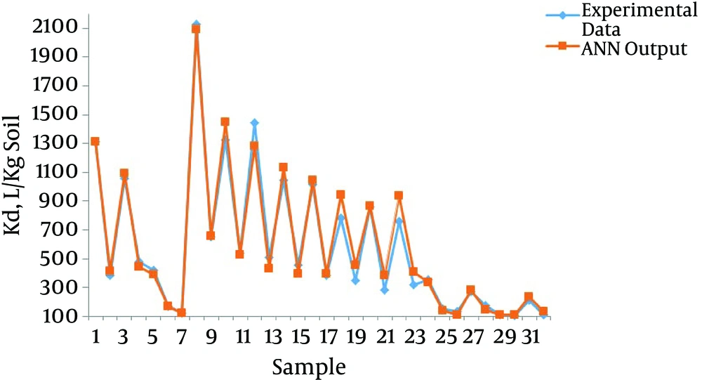
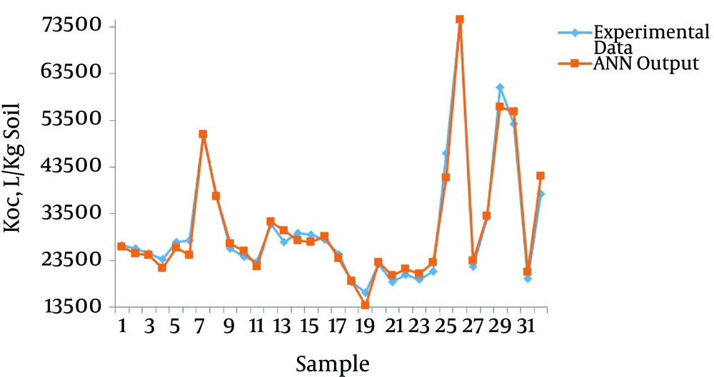
To evaluate the performance of the ANN model, the experimental data for Kd and Koc were plotted against the ANN output values (Figures 3 and 4, respectively).
After eight-fold cross-validation, the values of R2 and RMSE for Kd by the ANN model ranged from 0.92 to 0.99 and 15.67 to 110.79, respectively. These values ranged from 0.91 to 0.99 and 979.15 to 2655.84 for Koc (Table 3). Mean values for the eight networks used in the eight-fold cross-validation are presented in the last row of Table 3. The higher the R2 values, the more the precision of the model. Figures 3 and 4, Table 3 represent the most optimal accuracy of ANNs in predicting sorption coefficients. Low RMSE and high R2 values revealed the power of ANN in replicating and estimating the varieties of Kd and Koc of phenanthrene with soil organic carbon content variances, which demonstrated the strong correlation of Kd and Koc as the organic carbon of the soil.
| Networks | Kd, L/kg Soil | Koc, L/kg Soil | ||
|---|---|---|---|---|
| RMSE | R2 | RMSE | R2 | |
| Network 1 | 27.50 | 0.99 | 1063.99 | 0.92 |
| Network 2 | 25.15 | 0.99 | 1722.24 | 0.99 |
| Network 3 | 101.42 | 0.93 | 979.15 | 0.95 |
| Network 4 | 68.79 | 0.99 | 1698.87 | 0.91 |
| Network 5 | 96.91 | 0.92 | 1489.18 | 0.93 |
| Network 6 | 110.79 | 0.95 | 1417.57 | 0.95 |
| Network 7 | 22.62 | 0.98 | 2655.84 | 0.98 |
| Network 8 | 15.67 | 0.98 | 2535.79 | 0.97 |
| Mean | 58.61 | 0.97 | 1695.33 | 0.95 |
aRMSE: root mean square error, Kd: soil sorption coefficient, Koc: soil organic carbon sorption coefficient.
5. Discussion
The high correlation between soil sorption coefficients and soil organic carbon obtained in this study is in consistency with the findings of Wauchope et al. (11), Hwang and Cutright (40), Liyanage et al. (41), Wang and Keller (42), Ahangar (43), and Umali et al. (44), which showed that organic pollutants sorption increased with raising carbon content.
For examining the sorption of phenanthrene by heavy metals polluted soils, Gao et al. (45) reported a great variation for Koc values in different soils (5064-11461 L/kg), which was in agreement with results of the current study (high CV values). Such variation could be due to the nature of SOM and its compositional variances. In general, the effects of the nature or the site of SOM on the influential level of the active organic matter used to absorb PAHs were recognized (46, 47).
Gao et al. (14) conducted linear regressions with logKow, logS, and a combination of logKow and logS. Furthermore, they applied a nonlinear ANN to correlate Kow and S with Koc, and trained a simple neural network on Kow and S which was also obtained from the literature. The current study outcomes are similar to the results of these researchers, who found out that comparing with linear models, ANNs were more powerful in fitting the values of Koc and exhibited a lower sum of square residuals. High R2 values of resulted ANN networks in the research demonstrated that ANN was also accurate enough to estimate sorption coefficients. This could be due to the nonlinear relationships between the inputs and outputs, where in inputs there was a model less sensitivity to error. Furthermore, our findings are consistent with the results of Diaconu et al. (27), confirming the generalization ability of ANN to forecast the rate of adsorbed phosphate pollutant and its sorption volume on soil particles (with RMSE and R values of 0.929 and 0.987, respectively). They are also similar to the results of Snidgha (28) who reported the mean square error (MSE) value of 0.001 and R of 0.993 between the predicted and the observed values of neural network model on phenol pollutant. In this regard, Falamaki (13) used trained multilayer perceptron (MLP) and radial basis function (RBF) networks for estimating values of Kd for nickel, taking pH as input. He also found that MLP network could predict Kd better than RBF network and the results of all networks were superior to the linear models.
5.1. Conclusions
This study introduced the ANN approach as an efficient way for replicating and estimating the variability of phenanthrene Kd and Koc values related to soil organic carbon content. That is, Kd and Koc values are highly associated with this quality of soil. The best array used for ANN had one node in each input, one node in each output, and six nodes in each hidden layer. Furthermore, 1000 was the optimum value of iteration for the resulted structure in which tansig was selected as the most efficient transfer function. ANNs for Kd resulted in R2 and RMSE values ranging respectively from 0.92 to 0.99 and from 15.67 to 110.79 after eight-fold cross-validation. These values ranged from 0.91 to 0.99 and 979.15 to 2655.84 for Koc. In addition, this study claims that for the first time, the predicted phenanthrene sorption coefficients (Koc and Kd) have been used for the artificial neural networks, so the scholars have suggested ANN as a promising alternative for the conventional methods of estimating this pollutant, mainly because of the nonlinear and complex accounting relationships between the variables.


