1. Background
Child growth is often regarded as the best worldwide predictor of children's physical well-being since inadequate feeding habits, in both quantity and quality or, more frequently, a mix of the two, are vital factors influencing children's physical growth and mental development (1). Poor child development results from several issues that are inextricably tied to a population's general level of living and its ability to satisfy its fundamental requirements, such as access to food, shelter, and health care. As a result, child growth assessment serves not only as a tool for assessing children's health and nutritional condition but also as an effective indicator of community health disparities (2). Well-nourished children are more likely to grow into healthy adults. Globally, at least one in every three children under the age of five is no longer growing generally due to malnutrition in its most severe form of undernutrition (stunting, wasting, and underweight) (3).
This study focuses on a longitudinal study in which the outcome of interest is the children's body weight. Body growth is a positive change in body size over time and is a sensitive indicator of a child's health (1). Measurements such as height, weight, and head circumference are commonly used to assess a child's growth. Assessing a child's growth is a universal procedure to detect growth failure and its relationship to undesirable factors. Several studies in Ethiopia have investigated the impact of various factors on body weight, but investigating these impacts on their growth trajectories is limited (4-6).
2. Objectives
This study aimed to investigate variations in body-weight trajectories and the impact of distinct factors on the trajectories in a sample of Ethiopian children from infancy to 15 years.
3. Methods
3.1. Data and Study Participants
The longitudinal data were collected as part of the Young Lives cohort study, which is a 15-year longitudinal study that looks at the changing nature of childhood poverty in low- and middle-income countries. The outcome of interest for this study is the children's body weight repeatedly measured from ages 1 to 15 years, at ages 1, 5, 8, 12, and 15 years (7). This study included children who had weights measured five times between the ages of 1 and 15. Thus, 8,325 observations were obtained from 1,665 children (n = 5 observations for each). Formal ethical approval for this study was obtained from the Young Lives study, reviewed and approved by the Ethics Committee of Oxford University.
3.2. Description of Study Variables
Children's anthropometric measures were based on the World Health Organization standards (8, 9). The response variable was a child's weight measured by a scale (kg). The independent variables were gender, age, region, residence area (rural and urban), sleeping hours, father's level of education, father's age, mother's level of education, mother's age, household size, wealth index, and access to safe drinking water.
The wealth index is the primary indicator of households' socioeconomic position in the Young Lives sample. It is constructed based on housing quality, access to services, and ownership of consumer durables (10). The wealth index is calculated as a simple average of the three indices, assuming that its three components are equally important (11). The average yields a number between 0 and 1, with a greater wealth index indicating a better socioeconomic standing.
3.3. Statistical Analysis
Mixed-effect models are commonly used for modeling longitudinal data to test hypotheses regarding intra-individual changes and inter-individual variations in intra-individual changes (12, 13). Then, the linear mixed-effect (LME) model (14, 15) can be written as follows:
Where, yi is the (ni × 1) vector of continuous outcome for the ith individual, Xi is an (ni × p) covariate matrix related to the fixed effects β, where β ε Rp×1, Zi is the (ni × q) design matrix related to random effects bi, where bi ε Rq×1, and εi is the (ni × 1) within-individual error vector.
When the trajectory change is assumed to be linear, and the form of the shape is not debated, it is linear. However, when the change is non-linear, the trajectory shape is commonly chosen from various options. For example, Royston and Altman (16) presented fractional polynomial, which allows non-linear trajectories. The m-order fractional polynomial with power
j = (1, 2, …, m)
Where, p = (p1, …, pm) is a real-valued vector of powers,
The data were analyzed using SAS statistical software (version 9.4).
4. Results
4.1. Exploratory Analysis
Overall, 1,665 children with five times weight measurement were followed from infancy to 15 years. They consisted of 883 (53%) boys and 782 (47%) girls. Table 1 provides a more detailed explanation of the study variables and their frequency distribution. Table 2 shows the mean, variance-covariance, and correlation of weight measurements taken on the same child at ages 1, 5, 8, 12, and 15 years. The mean weight increases with age, but the increment rate is different. This indicates that a linear model is not applicable to model weight growth trajectories.
| Variables and Categories | No. (%) |
|---|---|
| Gender | |
| Boy | 883 (53) |
| Girl | 782 (47) |
| Residence area | |
| Rural | 1083 (65) |
| Urban | 582 (35) |
| Region | |
| Tigray | 356 (21.4) |
| Amhara | 272 (16.3) |
| Oromiya | 349 (21) |
| SNNP | 441 (26.5) |
| Addis Ababa | 247 (14.8) |
| Father's level of education | |
| Uneducated | 267 (16.0) |
| Grade 1 - 4 | 344 (20.7) |
| Grade 5 - 8 | 358 (21.5) |
| Grade 9 - 12 | 210 (12.6) |
| Diploma and above | 156 (9.4) |
| Adult literacy and religious | 330 (19.8) |
| Mother's level of education | |
| Uneducated | 612 (36.8) |
| Grade 1 - 4 | 320 (19.2) |
| Grade 5 - 8 | 281 (16.9) |
| Grade 9 - 12 | 149 (8.9) |
| Diploma and above | 69 (4.1) |
| Adult literacy and religious | 234 (14.1) |
| Access to safe drinking water | |
| Yes | 883 (53.0) |
| No | 782 (47.0) |
| Weight | Age 1 | Age 5 | Age 8 | Age 12 | Age 15 |
|---|---|---|---|---|---|
| Age 1 | 2.106 | 1.602 | 2.130 | 3.030 | 3.933 |
| Age 5 | 0.550 | 4.025 | 4.417 | 6.274 | 8.238 |
| Age 8 | 0.504 | 0.756 | 8.475 | 10.572 | 14.137 |
| Age 12 | 0.434 | 0.650 | 0.755 | 23.163 | 28.499 |
| Age 15 | 0.367 | 0.556 | 0.658 | 0.802 | 54.492 |
| Mean | 8.004 | 15.711 | 20.547 | 29.793 | 41.500 |
| SD | 1.451 | 2.006 | 2.911 | 4.813 | 7.382 |
a Variances on diagonal, covariances above diagonal, correlations below diagonal.
From Table 2, it can be observed that weight measurements performed on the same individual at different times are more likely to be correlated than measurements performed on different individuals, and two measurements taken close together on the same individual are likely to be more correlated than measurements taken further apart. Consequently, the correlated measurements must be considered at the time of analysis.
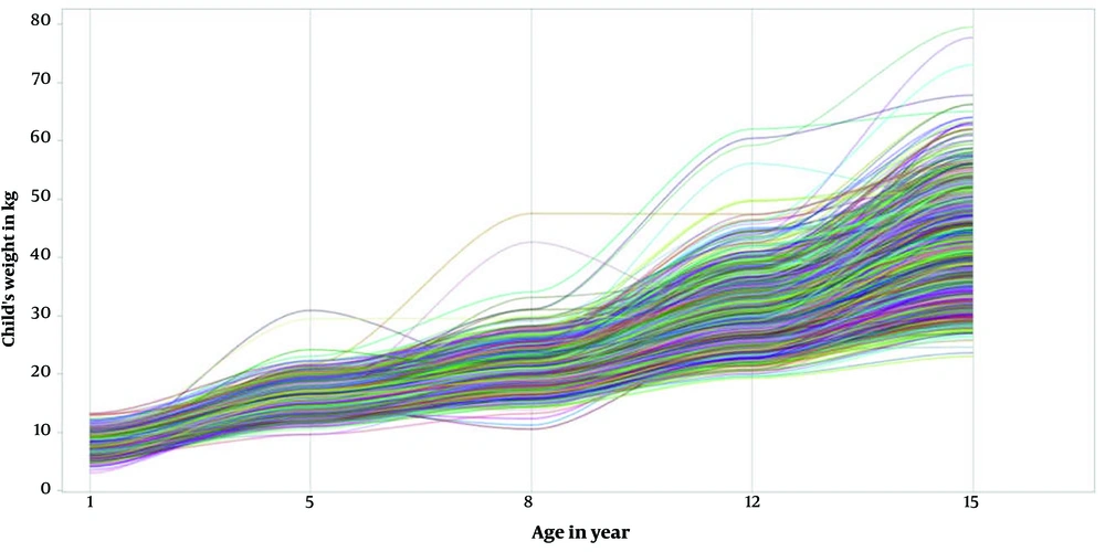
In addition to descriptive statistics, profile plots are essential in determining the functional form of the trajectories. Figure 1 depicts the plot of weight measurements against time for five waves of data. From this visual inspection, the between-individual variation is small in early childhood and increases with a child's age.
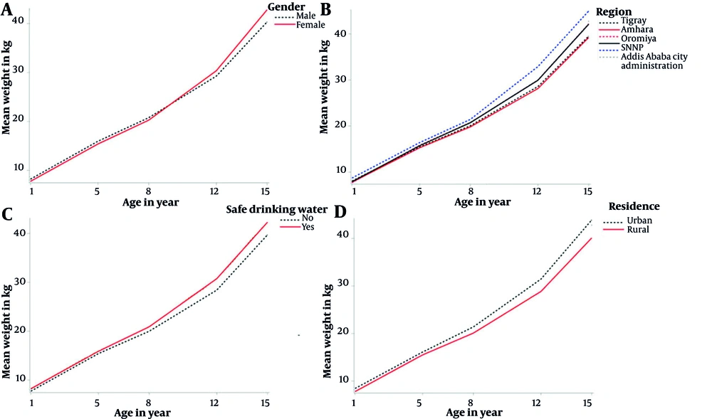
The mean profile plots against some covariates are given in Figure 2. Figure 2A signifies the growth curve for boys and girls. The weight growth curve by region of children is shown in Figure 2B. As depicted in this figure, children in Addis Ababa city had a higher mean weight in the entire period. In contrast, children in the Amhara region showed a slightly lower weight growth during the entire period. However, children in Oromiya and Southern Nations, Nationalities, and Peoples' Region (SNNPR) had similar growth fashions. The weight growth curve by safe drinking water is shown in Figure 2C. Children who had access to safe drinking water weighed more than those who did not. Figure 2D implies the weight growth curve by residence. It shows that urban children had a higher mean growth than rural children. From the results of descriptive statistics and visual inspections of the individual and mean profile plots, it is clear that the functional relationship between weight growth and time is not linear. Accordingly, a non-linear growth curve approach is a reasonable model for analyzing the weight data at hand.
The time variable was entered to model with single and combinations of power terms of p = [-2, -1, -0.5, 0, 0.5, 1, 2, and 3] and q = [-2, -1, -0.5, 0, 0.5, 1, 2, and 3]. Accordingly, a model with p = 0 and q = 3 revealed the lowest deviance. This suggests that the best-fitting second-order fractional polynomials were ln (age) and (age)3 based on deviance, Akaike, and Bayesian Information criterion statistics. Random effects were included for subject-specific intercepts and coefficients for age terms [ln (age) and (age)3] to allow body weight trajectories to vary across participants based on the likelihood ratio test of nested models. By using these power terms, a second-order fractional polynomial mixed-effect model is developed as follows:
The effects of fixed covariates such as a child's gender, area of residence, fathers' level of education, mothers' level of education, fathers' age, mothers' age, number of household sizes, wealth, access to safe drinking water, sleep duration in hours, and fractional polynomial function of time were included in the model and examined. The results of fractional polynomial mixed-effect models are presented in Table 3.
| Effect | Estimate | SE | t Value | Pr > |t| |
|---|---|---|---|---|
| Intercept | 9.4798 | 0.6496 | 14.59 | <0.0001 |
| Gender (girl) | -0.6859 | 0.1284 | -5.34 | <0.0001 |
| Residence (rural) | -0.02297 | 0.1827 | -2.13 | 0.0099 |
| Safe drinking water (no) | -0.1492 | 0.09902 | -1.51 | 0.1318 |
| Region (ref. = Tigray) | ||||
| Addis Ababa city | 0.3224 | 0.2646 | 3.46 | 0.0436 |
| Amhara | -0.4753 | 0.2196 | -1.16 | 0.3050 |
| Oromiya | 0.0601 | 0.2063 | 2.83 | 0.0068 |
| SNNPR | 0.1513 | 0.1934 | 3.78 | 0.0434 |
| Father's education level (ref. = uneducated) | ||||
| Adult literacy and religious education | -0.1728 | 0.1872 | -0.92 | 0.3559 |
| Diploma and above | 0.9785 | 0.3212 | 3.05 | 0.0023 |
| High school | 0.2381 | 0.2332 | 1.02 | 0.3072 |
| Primary school | 0.05352 | 0.1355 | 0.4 | 0.6928 |
| Mother's education level (ref. = uneducated) | ||||
| Adult literacy and religious education | 0.3396 | 0.2135 | 1.59 | 0.1118 |
| Diploma and above | 0.217 | 0.461 | 2.47 | 0.0379 |
| High school | 0.07059 | 0.2819 | 0.25 | 0.8023 |
| Primary school | 0.1706 | 0.1513 | 1.13 | 0.2597 |
| Household size | -0.07346 | 0.02611 | -2.81 | 0.0049 |
| Wealth | 1.4114 | 0.4088 | 3.45 | 0.0006 |
| Sleep duration in hours | -0.03639 | 0.03252 | -1.12 | 0.2632 |
| Father's age | -0.00734 | 0.01043 | -0.7 | 0.4816 |
| Mother's age | 0.1682 | 0.1491 | 2.13 | 0.0294 |
| Natural logarithm of time [ln (t)] | 3.8265 | 0.1901 | 20.13 | <0.0001 |
| Cubic time (t3) | 0.006386 | 0.000075 | 85.29 | <0.0001 |
a Time signifies the age of children, and SNNPR represents the southern nations, nationalities, and peoples' region.
Body weight changes significantly over time with natural logarithm [ln (t): 3.83, P < 0.0001], and cubic age (
The educational level of fathers and mothers is also associated with their children's weight. As shown in Table 3, the positive mean differences in weight growth between children of most educated parents and children of uneducated parents show that children of most educated parents (diploma or above-father: 0.979, P = 0.0023, diploma or above-mother: 0.217, P = 0.0379) had significantly higher mean weights than those from uneducated parents. However, there was no discernible difference in mean weight between children of uneducated parents and children of parents with less than a diploma qualification (father: adult literacy and religious education: -0.173, P = 0.3559, high school: 0.238, P = 0.3072, primary school: 0.054, P = 0.6928 and mother: adult literacy and religious education: 0.3396, P = 0.1118, high school: 0.0706, P = 0.8023, primary school: 0.1706, P = 0.2597). Furthermore, the relationship between mean weight and mother age is highly favorable, implying that a mother's age has a major beneficial impact on the child's growth (mother age: 0.1682, P = 0.0294). The age of a father, on the other hand, has no bearing on the child's development (father age: -0.00734, P = 0.4816). Household size has a significant negative effect (household size: -0.073, P = 0.0049) on child growth, while the wealth index has a significant positive effect (wealth: 1.4114, P = 0.0006). The amount of time children spend sleeping (sleep duration: -0.036, P = 0.2632) and safe drinking water access do not influence their body weight (safe drinking water: -0.149, P = 0.1318).
4.2. Rate of Changes in Body Weight Gain
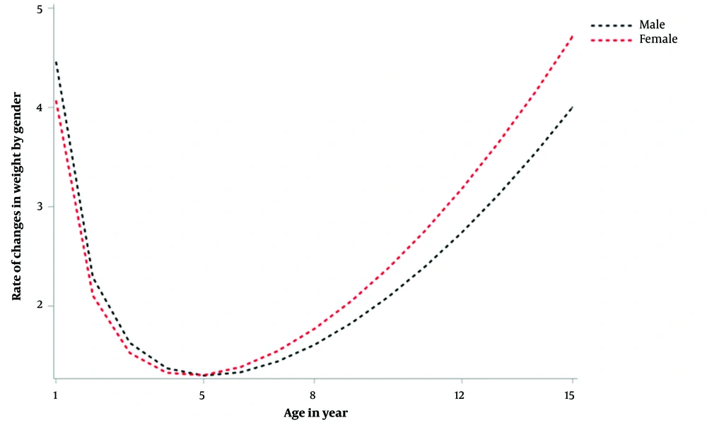
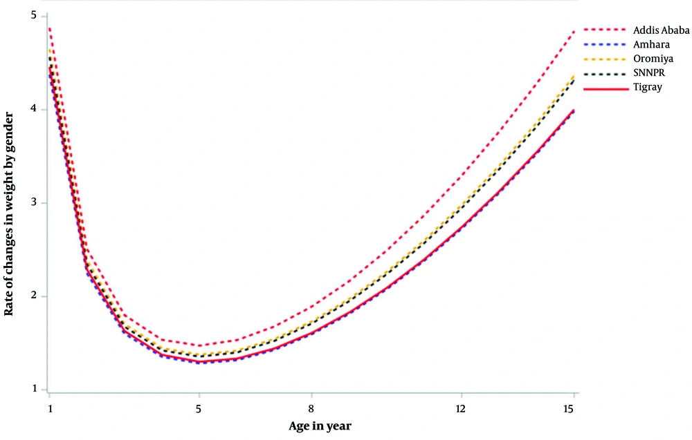
The mean differences are 7.71 between the first and second weight measurements, 4.84 between the second and third measurements, 9.25 between the third and fourth measurements, and 11.71 between the fourth and final measurements. The time adjacent increases in the means are not equal throughout time but are bigger in magnitude for the latter years than for the earlier years (Figure 3). This suggests that the weight gain curves are not straight. Accordingly, the natural logarithm and cubic age functions are the best fit for analyzing the nonlinearity weight growth trajectories over time. The mean of the natural logarithm factor is 3.8265, which corresponds to the slope of the tangent line of the curve at age one. On average, this suggests that children have a positive natural logarithm growth component in their trajectories. The mean of the cubic age factor is 0.006, suggesting that, on average, the curve increases as a child's age increases. These findings show that the developmental trajectory of the child's weight increases with time, with the degree of change rising as the children get older.
The rate of changes in weight gain was varied by gender and region. The interaction effects between these factors (gender and region) and age functions are presented in Table 4. There was a significant growth variation in weight across children from different regions of Ethiopia. Compared to the rate of weight gain of children in the Tigray region, the rates of change were significantly higher in children from Addis Ababa, Oromiya, and SNNPR. However, there was no variation in body weight changes between children in Tigray and Amhara regions. Boys had a higher rate of weight gain than girls. The rate of changes by gender and region are displayed in Figures 3 and 4, respectively. These figures exhibit that the rate of weight gain is more accelerated in the early and later years.
| Effect | Estimate | SE | t Value | P-Value |
|---|---|---|---|---|
| ln (age) × girl | -0.3941 | 0.05948 | -6.63 | < 0.0001 |
| age3 × girl | 0.0011 | 9.4E-05 | 11.63 | < 0.0001 |
| Region (reference group = Tigray) | ||||
| ln (age) × Addis Ababa | 0.4106 | 0.09736 | 4.22 | < 0.0001 |
| ln (age) × Amhara | -0.0837 | 0.09505 | -0.88 | 0.3786 |
| ln (age) × Oromiya | 0.1888 | 0.08926 | 2.12 | 0.0344 |
| ln (age) × SNNPR | 0.1028 | 0.08496 | 1.21 | 0.2264 |
| age3 × Addis Ababa | 0.0012 | 0.00015 | 7.84 | < 0.0001 |
| age3 × Amhara | -2E-05 | 0.00015 | -0.15 | 0.8805 |
| age3 × Oromiya | 0.00051 | 0.00014 | 3.72 | 0.0002 |
| age3 × SNNPR | 0.00046 | 0.00013 | 3.45 | 0.0006 |
5. Discussion
A longitudinal analysis was used in this study to look at the weight growth trajectory of children and the effects of various factors on their growth. The study identified that the functional relationship between weight growth and the age of children is non-linear. Age transformation is required to capture this nonlinearity trajectory in weight growth. As a result of a fractional polynomial approach, the best-fitting age transformation was identified, and the ln (age) and age3 power terms were chosen as the best-fitting functions of weight growth.
The findings showed that gender significantly affected the weight growth trend, with boys being significantly heavier than girls. This could be due to a genetic difference (17). This finding is consistent with previous studies that found boys were weightier than girls (1, 18). The results also demonstrated that the education of mothers and fathers had a significant impact on the children's weight growth, with children of more educated mothers and fathers being heavier than their counterparts, which agrees with the previous study, suggesting that infants of educated parents are heavier than their counterparts (19). The birth weight of children born to low-educated mothers was significantly lower than that of children born to higher-educated mothers (1). This is because parental education, either mother or father, and children's health outcomes is positively associated (20).
The study revealed that sleeping hours and the father's age had no significant effect on the growth trends, consistent with the previous studies showing that the parent's age had no significant effect on the child's growth trajectory (21). There was no statistically significant relationship between children's sleep duration and assessed weight status (22). Furthermore, household size was negatively associated with the child's growth trend, while wealth was positively associated with the child's growth trend; this confirms the results of previous studies reporting that household structure was related to children's concurrent stunting and overweight (23). In addition, the residence area (urban and rural) had a significant effect on the weight gain trend; this suggests that children in urban areas were significantly heavier than those in rural areas, supporting previous research findings (21). The difference in growth between children in urban and rural areas could be due to socio-environmental factors and nutritional status (6, 13). The rate of weight gain was varied by region. The rates of weight gain of children in Addis Ababa, Oromiya, and SNNPR were greater than that of children in the Tigray region. There was no difference in body weight changes between children in Tigray and the Amhara area.
A child's weight was measured repeatedly over time, and these measurements are correlated. In such circumstances, a model that appropriately accounts for the correlated measurements is critical for estimating parameters and testing hypotheses. Longitudinal studies are more successful and have more statistical power in studying changes over time (24, 25). The strength of longitudinal studies over cross-sectional studies is their ability to analyze the individual growth of a certain outcome variable across time (1, 26). One weakness of this study was that it was limited to five regions of Ethiopia; hence, it may not be representative of the entire population of Ethiopian children. As a result, further study on Ethiopian children is required to discover the most critical influence of crucial variables.
5.1. Conclusion
The findings showed that while controlling for other factors, gender, residence, region, parental education, household size, wealth, and mother's age had a significant influence on the longitudinal weight growth of children. However, safe drinking water, sleeping time, and father's age were not related to the weight trajectory over time. The growth rate in weight was accelerated in the early and later years.
