1. Background
Cardiac magnetic resonance imaging (CMRI) is an accurate and reproducible technique for the evaluation of cardiac function. It is also the gold standard for ventricular volume measurements as documented by both ex vivo and in vivo studies (1). Left ventricle volume measurement needs segmentation of the left ventricle (LV), which is a difficult task because of its unclear borders and shape variety. The presence of papillary muscles in the ventricle cavity, with gray level values similar to the surrounding myocardium is considered as another problem. In summary, the problem of left ventricle segmentation is still open due to these issues; whereas, numerous methods have been proposed (2, 3). The previous works may be categorized into different groups: active contour (4-6), methods based on computation of thresholding (7, 8), graph search algorithms (9, 10), atlas based methods (11-14), and statistical shape models (active shape and appearance model) (15-17). Among these methods, statistical shape models are the most used approach in this field (2, 3). Atlas-based segmentation uses labeled images, known as atlas, to describe diverse structures present in the intended image. Registration of atlases onto the image to be segmented is the key point of this procedure (3). As literature shows (2, 3), the main drawback of this method is the effect of the registration quality on the success of the approach. Active contour is another approach of medical image segmentation that has been widely used regarding their flexibility (18). Active contours are iteratively deforming curves that minimize an energy functional with their evolution, and meanwhile use information of object boundaries and smoothness of curve as separate terms (2). A number of methods have been worked on using active contour model for left ventricle segmentation. Grosgeorge et al. (5) utilized well-known region based active contour approach, Chan-Vese approach, for segmentation of both left and right ventricle. Their results show a satisfying segmentation, but because of using region term solely, this method results good only in homogenous regions with well-defined borders. Graph based method is another approach used for right and left ventricle segmentation. In graph-based methods, every image pixel is considered as node and edges between graph nodes are defined with similarity function. Cut is a set of edges of graph that omitting them partitions the graph into two disjoint sets. Global optimization of cost function is the framework of this approach. Graph theoretic techniques are not limited to graph cut and generally are categorized into four groups (19): (1) Graph cut: Cuts can be obtained using minimizing a predefined cost function or on Markov random field models. (2) Minimum path based methods: These methods are semi-automatic approaches that define the object frontiers as minimum cost paths between each pairs of nodes. (3) Methods based on minimal spanning tree: A minimum spanning tree (MST) is a tree of a connected undirected graph that connects all the vertices together with the minimal total weights for its edges. For segmentation by this approach, edges from different sub-graphs are removed. (4) Other methods: graph based segmentation methods that are not part of any of the above categories (20). Among these four approaches, minimum path based method is considered as a semi-automatic technique. So, it is more interesting in medical applications because incorporating radiologist knowledge makes the segmentation process more reliable and accurate. The most well-known algorithm for solving “minimum path finding problem” is Dijkstra’s algorithm (21), which is also utilized in livewire (22). 2-D livewire method provides the possibility of selecting an initial point on the boundary of the object to be segmented. The next point is placed in a way such that the lowest cost path between the initial point and the current cursor position will find the object of interest interactively. There are efforts for extending 2-D livewire to 3-D framework (23-25) in various applications, especially medical applications. Another extended version of live wire is proposed in a study conducted by Poon et al. (26), in which the cost function is modified so it can segment vessel images more appropriately. They added vesselness filter, vessel direction term and fitness of medial node term to the livewire cost function. This idea actually works well in the 2-D segmentation context. Classical livewire hires image features like edge and gradient information, while this information in the ventricle border is inaccessible more often due to ill-defined borders and partial volume effect.
2. Objectives
We have used a simple region-based shape prior term for representation of the left ventricle. The shape prior, which is named LVness (a term that represents the shape of the LV), is based on a region growing algorithm that we previously presented (27). LVness produces a primary segmentation of the left ventricle according to region information. The resulted border pixels have low intensity values and guide the minimum path search algorithm to the predefined band. In the following, first we will describe the livewire approach and LVness generation procedure. The qualitative and quantitative results of applying proposed method on 45 cases of MRI images of a publically available dataset (MICCAI 2009 left ventricle segmentation challenge) is presented in the next section. Finally, discussion, conclusion and suggestions for future researches are presented in the later section.
3. Materials and Methods
3.1. Livewire
Livewire algorithm is a semi-automatic tool for accurate segmentation that gives the seed from user input. As the user selects seed points, and moves the mouse, optimal boundaries are computed and found. The classic 2-D livewire uses the gradient magnitude fm(q) gradient direction fd(p,q), and canny operator fc(q) for creating cost function from pixel p to pixel q C(p,q) (24).

Where wM, wD and wC are gradient magnitude, gradient direction, and edge detection weights respectively. These weights provide the possibility of contribution to the cost function with various rates for each cost term. The gradient magnitude is defined as:

In this equation, G refers to gradient magnitude in the 2D image and max (G) represents the largest gradient magnitude. As it is clear, gradient magnitude has high value in borders and low value in homogenous regions. As mouse moves around the object, the border pixels should have low costs so livewire algorithm can tend to the border. It’s obvious that gradient magnitude must be inverted and this provides low cost for strong edges. The gradient direction cost term pixel p going to pixel q is defined as:

Where G(p) represents the gradient magnitude for pixel p. Finally, fc(q) is the canny edge detector (28). Canny edge detector results a binary image with white pixels (it means 1) representing edges and black pixels (it means 0) are background.
Classical livewire hires image features like edge and gradient information, while this information in the left ventricle border is inaccessible more often due to ill-defined borders of LV in these images. Therefore, we used a shape prior term to be added to the cost function of minimum path search algorithm.
3.2. LVness
Here, we have defined a new term to be added to the cost function and incline the path toward the left ventricle. The new cost function forms as follows:

Where wLV indicates the weight of LVness term on the equation. For providing LVness by primary segmentation, we have used our previously presented region-based segmentation approach. First, the user selects a seed in the left ventricle region manually and afterward gray space map is formed.
3.3. Gray Space Map
Gray space map composition contains four major steps:
1) The coordinates and gray level value (V) of a seed is obtained by clicking on the left ventricle region.
2) Pixels that have the same gray level value as the seed and are neighbors of the seed pixel are found.
3) At this step, we define a set of gray levels in the interval [V - D, V + D], D ε {1, 2, … } and look forward pixels in the neighborhood of the previous step and with gray level value in this interval.
4) Every time D increases, corresponding pixels in gray space map catch a lower label.
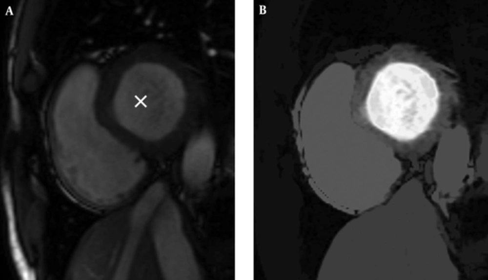
So, we have an image with the same size as the original image and pixels that are close to the seed (in terms of spatial and gray level value) are highlighted with higher values. Resulted gray space map is demonstrated in Figure 1.
3.4. LVness Generation
Regarding left ventricle prominence in gray space map, which is because of the homogeneous region of the left ventricle and inhomogeneity between LV cavity and surrounding tissues, a robust method is needed to express left ventricle edges as a weighted map like other terms of classic livewire. We have used the antepenultimate (two before the last) stage of canny edge detector (28), in which the edges are described as a weight of edgeness. The canny edge detector has five steps (28).
1) Image smoothing by applying Gaussian filter in order to remove undesired noises. An example of a Gaussian kernel of size = 5 and σ = 1.4 is represented in the following Equation. The The asterisk denotes a convolution operation.

2) Finding the intensity gradient of the image. The canny algorithm first finds horizontal and vertical gradients (Gx and Gy, respectively) using first derivative operators like Sobel. From this the edge gradient and direction can be determined according to the following Equation:

3) Apply non-maximum suppression, which is an edge thinning technique, to remove pixels that are not considered to be part of an edge. Hence, only thin lines (candidate edges) will remain.
4) Exert double threshold to determine potential edges. After application of non-maximum suppression, there are still some edge pixels caused by noise and gray level variation. In order to throw away these artifacts, it is essential to filter out the edge pixel with the low gradient value and preserve the edge with the high gradient value (29).
5) Hysteresis: canny uses lower and upper thresholds (T1 and T2, respectively):
- If: pixelGradient > T2
Then: the pixel is accepted as an edge.
- If: pixelGradient < T1
Then: the pixel is rejected.
- If: T1 < pixelGradient < T2
Then: the pixel will be accepted only if it is connected to a pixel that is above T2
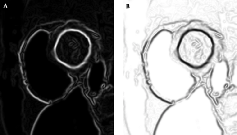
In these steps, the third step (i.e. non-maximum suppression) produces an image, in which pixels that have a weight according to “being edge” rate and on the other hand, undesirable noises are suppressed. If we stop canny algorithm in this step and use weights of this image as a criterion that represents LV border rate in the mouse-moving path, this output can be our LVness.
There is only another step for preparing our LVness and this would be complementing the resulted image. As Figure 2 shows, result of non-maximum suppression algorithm has higher values in more likely edge pixels and lower values for rest of pixels. For being minimum fLV near the left ventricle borders, it should be complemented as it can be seen in Figure 2.
Like other terms in the classic livewire, this new term is an image that has weights that are low values around the borders and high in the rest of the image pixels. As mathematically described above, all terms of modified livewire are images that would be minimum in the mouse-moving path around the LV border. Non-maximum suppression (NMS) has a derivative nature that arises from directional first order derivatives (Gx and Gy), and these operators has maximum in high variations (likes edges) according to following Equations:


This shows that fLV, which is the complement of NMS, is minimal near the borders.
3.5. Graph Searching Algorithm
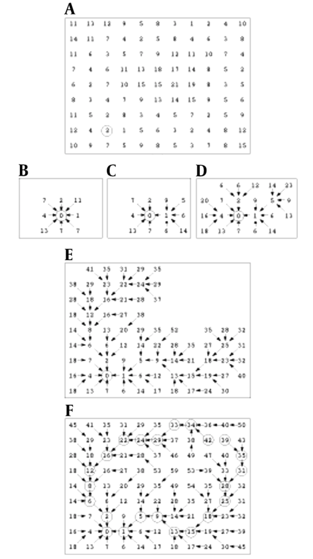
Finding a low cost path in our directed graph is the next task. Local costs are assigned to nodes in the graph and then, expansion of a user-selected seed point is accrued and it means that its local cost is added into its neighboring nodes. The next pixel, which is expanded, is the neighboring node with the minimum cumulative cost and the process continues till a “wavefront” is produced that expands in order of minimum cumulative cost (22). Figure 3 illustrates the described algorithm. Figure 3A shows the seed point with a circle around it and initial local cost map.
Figure 3B demonstrates a portion of the total cost after the seed point is expanded. Note that diagonal costs have been multiplied by Euclidean distance. Figure 3C indicates two points expansion, and Figure 3D-3F show 5, 47 and completed expansion (22).
3.6. Ethical Approval
This article does not contain any studies with human participants or animals performed by any of the authors.
3.7. Informed Consent
Informed consent was obtained from all individual participants included in the study.
4. Results
To evaluate the performance of the proposed method, we applied it to the MICCAI 2009 LV segmentation challenge dataset (3). The database is publicly available online and contains 45 MRI datasets, grouped into three categories. Each category contains 15 cases of ischemic heart failure cases, non-ischemic heart failure cases, LV hypertrophy cases and normal (SC-N) cases. Manual segmentation of images by experts at the end diastole (ED) and the end systole (ES) cardiac phases are available.
4.1. LVness Generation
LVness is built for ED and ES phases of cardiac cycle separately. There are also six LVness models for ED phase from base to apex and six for ES. Livewire cost function terms have weights that are chosen empirically from training sets: WM = 0.3, WD = 0.39, WC = 0.17 and WLV = 0.14. These weights are obtained empirically and WLV is set to 0.14 to suppress the effect of LVness in case of possible leakage of GSmap outward of the left ventricle. We have done sensitivity analysis to determine the change in accuracy while varying each weight value (30). We found that varying each weight by ± 50% did not change the accuracy by more than 4.3% for our test images. For more certainty in this matter, we performed a leave-one-out (LOO) strategy and in each iteration, one of the training, online and validation datasets of the MICCAI 2009 LV segmentation challenge dataset was considered as test group.
4.2. Quantitative and Qualitative Evaluation
Two well-known measures were used to analyze the performance of our segmentation approach with other methods that used dataset (3) dice metric (DM) and average perpendicular distance (APD).
The dice metric is a statistic that measures contour overlap by intersecting automatically segmented area and manually segmented area , multiplyed by 2, and finally divided by AA + AM (3).

The dice metric is always between zero and one, and higher DM shows better consistency between automated and manual segmentations.
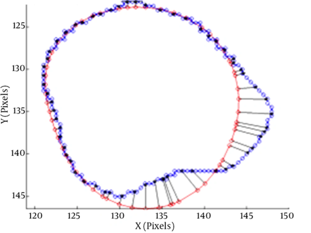
The average perpendicular distance measures the distance from the automatically segmented contour to the corresponding manually drawn expert contour, averaged over all contour points (3). A representation of APD can be seen in Figure 4.
The average perpendicular distance APD between two contours (3)
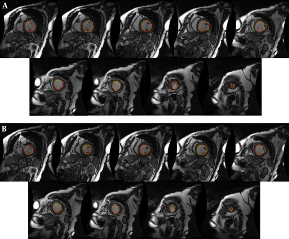
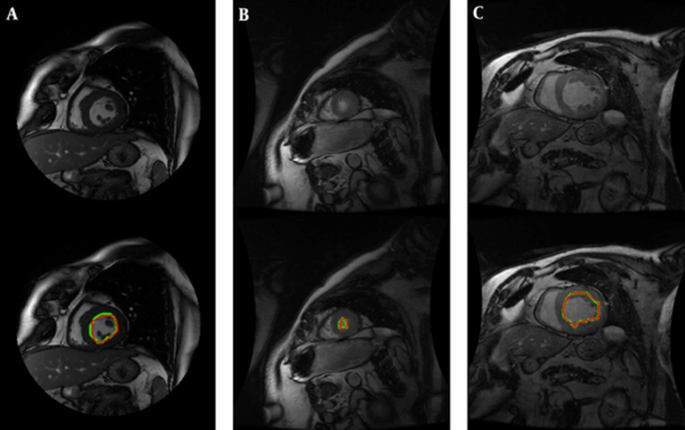
We have performed our segmentation algorithm on training, validation and online sets of dataset. The qualitative and quantitative tests show promising results. In comparison with other automatic and semi-automatic methods, our proposed method yielded the best results in both gice metric and APD and may be considered as state of the art. Table 1 shows the average values ± the standard deviation of the statistic measurements. Figure 5 illustrates the automatic and manual segmentation results of the LV from the base to the apex and also in ED and ES phases of the cardiac cycle. Segmentation of the left ventricle has pre-mentioned difficulties and these difficulties are boosted in mid and apex slices due to their low resolution and presence of papillary muscle. The ability of our method in segmentation of the left ventricle in these cases is presented in Figure 6.
| Dataset | DM | APD | |
|---|---|---|---|
| Training | ED | 0.95 ± 0.26 | 1.48 ± 1.32 |
| ES | 0.89 ± 0.11 | 6.23 ± 4.33 | |
| Validation | ED | 0.92 ± 0.19 | 4.11 ± 1.19 |
| ES | 0.90 ± 0.12 | 4.77 ± 0.12 | |
| Online | ED | 0.88 ± 0.34 | 3.45 ± 0.79 |
| ES | 0.86 ± 0.29 | 5.83 ± 2.35 |
Abbreviations: APD, average perpendicular distance; DM, dice metric; ED, end diastole; ES, end systole.
aValues are expressed as mean ± standard deviation.
Manual (red) and proposed approach (green) segmentation of the left ventricle from base to apex for an instance case of MICCAI 2009 challenge database (3). A, End diastole; B, End systole.
We have used MATLAB 2015-b with License-number: 838860 in a Pentium-4 system with Intel(R) Core(TM) 2 Dou CPU 2.80 GHz 8 GB RAM, 64-bit Windows 7.
5. Discussion
In this study, we developed and validated a new semi-automatic approach for left ventricle segmentation based on 2-D livewire. As classic livewire uses image features like gradient and edge information, and this information is not sufficient or inaccessible in some cases, we used our previously presented region growing algorithm to generate a primary segmentation that could be added as a new term to the livewire equation. Ideally, incorporating all regions, shape and edge information of the left ventricle may produce a fully promising result in left ventricle segmentation. However, incorporating all of these information needs a huge dataset that can capture all the shape varieties in the left ventricle. Computed metrics in Table 1 showed that our approach results provided contours similar to the ground truth by a rate of 93% and improvements in other metrics. Table 2 revealed that our method outperformed the state-of-the-art methods that used the same dataset (3). In Table 2, a comparison of results between our method and the state-of-the-art methods that used the same database is presented. The results show a significant improvement in both dice metric and average perpendicular distance by our proposed method. Figure 5 shows a greet agreement between our proposed method segmentation results and manual segmentation as ground truth. Figure 6 illustrates the ability of proposed method in segmentation of the left ventricle along with whole slices of end diastolic and end systolic phases of the cardiac cycle. In this figure, manual segmentation is declared by red contours and livewire segmentation by green contours. The conformity of manual and livewire segmentation can obviously be seen in all frames.
| Method | DM | APD |
|---|---|---|
| Proposed method | 0.95 ± 0.26 | 1.48 ± 1.32 |
| Classic livewire (22) | 0. 88 ± 0.22 | 8.13 ± 3.87 |
| Oghli et al. 2013 (31) | 0.79 ± 0.33 | 9.12 ± 1.23 |
| Oghli et al. 2012 (32) | 0.73 ± 0.56 | 9.58 ± 2.19 |
| (Queiros et al. 2014) (33) | 92.7 ± 0.23 | 10.51 ± 9.17 |
| (Ngo and Carneiro, 2014) (34) | 93.23 ± 0.34 | 22.20 ± 21.74 |
| (Hu et al. 2013) (35) | 0.61 ± 0.29 | 15.08 ± 8.91 |
| (Constantinides et al. 2012) (36) | 0.80 ± 0.19 | 9.79 ± 5.38 |
| (Jolly et al. 2009) (37) | 0.88 ± 0.04 | 2.97 ± 0.38 |
| (Liu et al. 2012) (38) | 0.78 ± 0.20 | 9.26 ± 4.93 |
| (Huang et al. 2011) (39) | 0.81 ± 0.16 | 7.28 ± 3.58 |
| (Schaerer et al. 2010) (40) | 0.77 ± 0.16 | 9.64 ± 4.15 |
Abbreviations: APD, average perpendicular distance; DM, dice metric.
aValues are expressed as mean ± standard deviation.
The most challenging slices for cardiac MRI segmentation could be divided in three groups:
1) Apical slices,
2) Slices with strong papillary muscles
3) Slices with an unclear border.
Figure 6 shows the robustness of the proposed method in segmentation of these challenging slices.
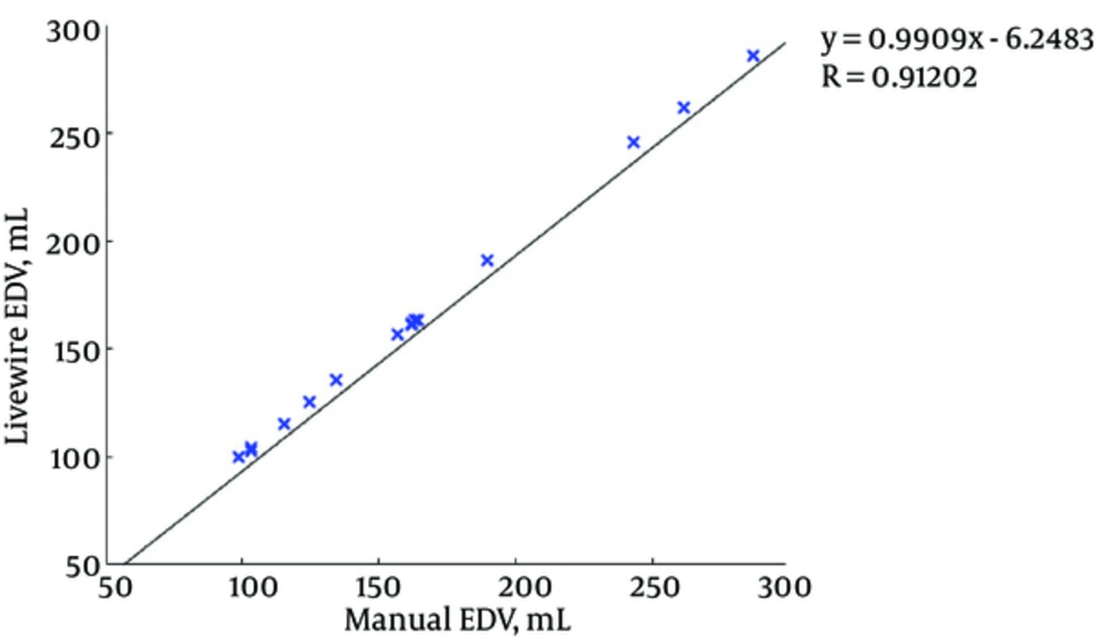
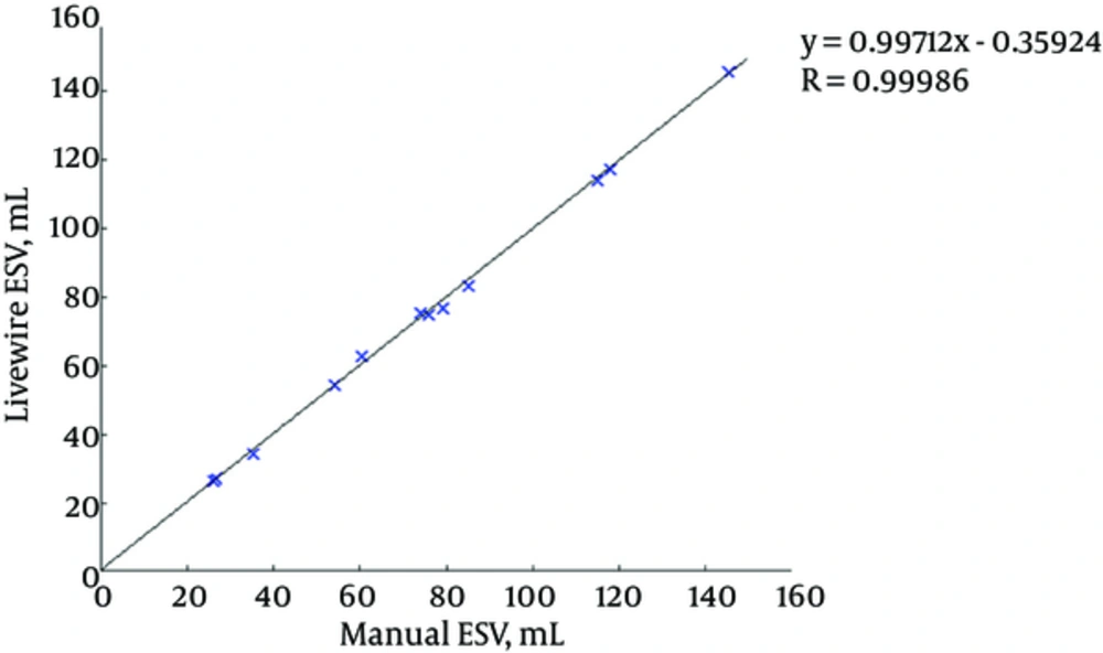
Figures 7 and 8 illustrate the correlation graphs using online data set between our approach and manual results for end diastolic and end systolic volumes, respectively. A correlation with manual segmentation of 0.997 and 0.997 for end-diastolic volume (EDV) and end-systolic volume (ESV) was calculated. The correlation test is obtained using “Pearsons test” to obtain the slope, intercept and the R-values. This high correlation proves the accuracy and clinical applicability for evaluation of LV function.
We used a 2-D approach for segmentation of the left ventricle; whereas, 3D methods are becoming the state-of-the-art in medical applications, and this is because of two reasons:
1) The large gap between slices in short axis and other views (about 7 mm) and impossibility of the pixel intensity value estimation in the gaps (2, 3).
2) Misalignment between slices due to motion artifacts in cardiac MRI (25). This means that the cavity center is not at the same position in different slices.
Among various methods that are used for left ventricle segmentation in the literatures, active contour methods (especially level set based method) and active shape and appearance methods (active shape model (ASM) and active appearance model (AAM) are the mostly used approaches. Level set based methods uses an initial contour and aggregate edge information (and in some cases like Chan-Vese region information) to minimize a function that leads to evolve a curve to fit on object boundaries. Besides their significant advantages, these methods have the following limitations:
1) The main disadvantage of this approach is the dependence of segmentation result to precision of initial contour selection. Although this weakness is mostly resolved, the problem is still open.
2) They can often get stuck in local minimal states; this may be overcome by using simulated annealing techniques, which is the cause of computational complexity.
3) Accuracy is governed by the convergence criteria, which is used in the energy minimization technique. Higher accuracy require tighter convergence criteria and hence, longer computation times.
4) Another issue that makes the use of level set methods for LV segmentation inappropriate is the presence of papillary muscles with gray levels similar to surrounding myocardium. These little circle shaped muscles (which are obvious in Figure 5A) create local minima for evolving curve because of edges that are between them and LV cavity.
It is notable that although the proposed method (base on livewire framework) is a semi-automatic approach as level set method, there are some differences between user interaction in the proposed method and level set approach. The main difference is that in livewire method, user selects the seeds exactly on the left ventricle border and since the operators are expert (or at least semi-expert) they recognize ventricle positions and user interaction will not result in miss-segmentation or user faults. On the other hand, the shortest path between two seeds is recognized based on livewire algorithm and is confirmed by selecting the next seed by the user. While, in the level set method user selects an initial contour and the contour evolves based on an energy minimization algorithm. This fact limits the supervision of the user and may lead to miss-segmentation in some cases.
Active shape and appearance methods hire a point correspondence based method [point distribution model (PDM)] for representation of left or right ventricle shape. ASM captures shape variations, constructs a model and aims to match the model to a new image. On the other hand, AAM works with shape and appearance of object simultaneously based on correspondent points (15). The main drawback of these techniques is the dependence of the result of segmentation on the similarity of shapes to the training set.
5.1. Conclusions
In summary, a combined semi-automatic approach for segmentation of the left ventricle is proposed in this paper, which incorporates region information with a region-growing algorithm into the livewire framework. In contrast to automatic manners, semi-automatic approaches in image segmentation has the advantage of using knowledge and experience of a radiologist. This superiority is more essential in cardiac MRI image analysis, which has a lot of ambiguities in interpretation of the image. On the other hand, the time spent for segmentation of a single slice is very lower than manual segmentation.
