An Efficient Method for Automated Breast Mass Segmentation and Classification in Digital Mammograms

Behrouz Niroomand Fam; Alireza Nikravanshalmani; Madjid  Khalilian

doi:10.5812/iranjradiol.106717

An Efficient Method for Automated Breast Mass Segmentation and Classification in Digital Mammograms

authors:

Behrouz Niroomand Fam ¹ , Alireza Nikravanshalmani ^{1
, *} , Madjid Khalilian ¹

1 Department of Computer, Karaj Branch, Islamic Azad University, Karaj, Iran

how to cite: Niroomand Fam B, Nikravanshalmani A, Khalilian M . An Efficient Method for Automated Breast Mass Segmentation and Classification in Digital Mammograms. I J Radiol. 2021;18(3):e106717. https://doi.org/10.5812/iranjradiol.106717.

Abstract

Background:

Automatic detection and classification of breast masses in mammograms are still challenging tasks. Today, computer-aided diagnosis (CAD) systems are being developed to assist radiologists in interpreting mammograms.

Objectives:

This study aimed to provide a novel method for automatic segmentation and classification of masses in mammograms to help radiologists make an accurate diagnosis.

Materials and Methods:

For an efficient mass diagnosis in mammograms, we proposed an automatic scheme to perform both mass detection and classification. First, a combination of several image enhancement algorithms, including contrast-limited adaptive histogram equalization (CLAHE), guided imaging, and median ﬁltering, was investigated to enhance the visual features of breast area and increase the accuracy of segmentation outcomes. Second, the density of discrete wavelet coefficient density (DDWCs), based on the quincunx lifting scheme (QLS), was proposed to find suspicious mass regions or regions of interest (ROIs). Finally, mass lesions that appeared in the mammogram were classiﬁed into four categories of benign, probably benign, malignant, and probably malignant, based on the morphological shape. The proposed method was evaluated among 1593 images from the Curated Breast Imaging Subset-Digital Database for Screening Mammography (CBIS-DDSM) dataset.

Results:

The experimental results revealed that the suspected region localization had 100% sensitivity, with a mean of 6.4 ± 4.5 false positive (FP) detections per image. Moreover, the results showed an overall accuracy of 85.9% and an area under the curve (AUC) of 0.901 for the mass classification algorithm.

Conclusion:

The present results showed the comparable performance of our proposed method to that of the state-of-the-art methods.

Keywords

Breast Mass Computer-aided Diagnosis Image Processing and Analysis Mass Classification

1. Background

Breast cancer has currently become one of the main global health challenges and the first cause of cancer-related mortality in women worldwide. According to the World Health Organization (WHO), there were more than two million newly diagnosed breast cancer cases in 2018 (11.6% of all cancers). This type of cancer is also the fourth leading cause of death, accounting for 626,679 deaths in 2018 (1). A screening mammogram is the most effective method to reduce the mortality of breast cancer and increase the survival rate by early detection. However, the interpretation of mammograms is often a challenging task, and radiologists may misdiagnose a large proportion of cases. Masses and calcifications are the most common types of abnormalities in mammograms. Also, masses are similar to some breast tissues and can be located in dense areas of breast tissues, making it difficult to detect them. These issues make breast mass detection a challenging problem for both radiologists and computer-aided diagnosis (CAD) systems.

In recent years, many studies have been conducted on the development of CAD systems for breast cancer detection (2-4). Most of these studies are completely dependent on segmentation and hand-crafted features, which are not optimal. In some studies, wavelet coefficients and features extracted from wavelet coefficients have been used to detect breast abnormalities in mammograms (5, 6). In these methods, it is necessary to define hand-crafted features to detect and classify mass regions in mammograms; therefore, the performance of these methods is limited. Besides high computational cost (7), these methods have resulted in a rather signiﬁcant number of false-positive (FP) results (8).

More recently, deep learning-based approaches, especially convolutional neural networks (CNNs) (9-11), have been introduced to overcome these limitations. However, they require large annotated datasets for training, which are expensive and time-consuming to acquire. Moreover, training a CNN requires a massive amount of data, a high computing power, and large memory resources. Some studies have used morphological features to distinguish benign tumors from malignant ones (12-14). Benign masses are round or regular, smooth, and well-defined, while malignant masses have much more irregular, rough, spiculated, or blurry boundaries. In this regard, Liu and Zeng (15) extracted various types of hand-crafted features from ROIs and fed them into a support vector machine (SVM) for classification. Masses were detected with 82.4% sensitivity and 5.3 false positives per image (FPPI), using the digital database for screening mammography (DDSM) database.

In another study, Vadivel and Surendiran (12) used shape and margin features to develop an approach for mass classification in mammograms and examined this approach in the DDSM database. The classification results showed an accuracy of 87.76%. More recently, Shen et al. (9) proposed a new deep learning framework for detecting and classifying breast masses. They achieved the best performance with a true positive rate (TPR) of 0.812 and false positives per image (FPI) of 2.53 on the CBIS-DDSM database. So far, although various methods have been developed for breast mass classification, accurate classification of malignant and benign masses is still a major challenge.

2. Objectives

In this study, for an accurate and efficient mass detection in digital mammograms, we proposed a density of discrete of wavelet coefficient (DDWC)-based method for localizing suspected lesions on mammograms. The masses appearing on mammograms were further analyzed and classified into four groups based on the morphological features.

3. Materials and Methods

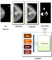
In this study, the proposed method was divided into two main stages. The first stage was related to the detection of suspicious mass regions on mammograms, while the second stage was related to the classification of these regions as benign, probably benign, malignant, and probably malignant. The steps of the proposed method are presented in Figure 1. Each step will be described in the sections below.

Figure 1.

The schematic diagram of the proposed method for breast mass detection and classification based on the input digital mammogram

3.1. Pre-Processing Stage

Figure 2 presents the pre-processing stage, which includes four phases. In the first phase, unwanted portions, such as borders, labels, and additional artifacts, are removed from the normalized grayscale mammogram, and the breast area is segmented. In the second phase, the denoising process was used to highlight some information about tissues contained in the mammogram. The third phase was image enhancement, which allowed for a better visualization of speciﬁc regions (e.g., abnormalities) in the image. Moreover, contrast-limited adaptive histogram equalization (CLAHE) and morphological operations were used to further enhance the mammographic image and reduce the noise produced in homogeneous areas. In the final phase, guided image filtering was performed to obtain a refined mammogram. The pre-processed mammogram M_p was used as input for the segmentation stage, as shown in Figure 3.

Figure 2.

The block diagram of the pre-processing stage

Figure 3.

An example of applying the suspicious region localization (SLR) method in a mammogram. A, Original mammogram and red rectangle is the area containing the mass; B-F, The pre-processing step: B, Removal of noise and radiographic artifacts and selection of the breast region, C, Morphological operation; D, Wavelet denoising; E, Contrast-limited adaptive histogram equalization (CLAHE); and F, Guided Image filtering; G, Segmentation based on the quincunx lifting scheme (QLS) and post-processing; and H, The final results and mask image (ROI).

3.2. Suspected Region Localization (SRL)

In this stage, the pre-processed mammogram, obtained from Section 3.1, was used as the input. This study focused on finding suspicious regions (SRs). Generally, analysis of mammograms is a difficult task due to the irregularity of mammogram texture. Since mammography is a non-stationary signal, discrete wavelet transform (DWT) (16) is an efficient tool for analyzing different signal components at different resolution scales. A signal in wavelet decomposition can be represented as follows:

Equation 1.

F (t) = \sum_{i} \sum_{j} c_{i j} φ_{i j} (t)

where $φ_{i j} (t) = 2^{\frac{i}{2}} φ (2^{i} t - j)$ and $φ_{i j} (t)$ are the basic functions, and c_ijis a coefﬁcient (a numerical value). The information and nature of a given signal are determined by the coefﬁcients since the basic functions are ﬁxed. Also, the Fourier transform $x ̂ (ω)$ of x is deﬁned as follows:

Equation 2.

\hat{x} (ω) = \sum_{n ϵ Z^{2}} x [n] e^{- j ω^{T} n}

where zⁿ = $Z_{1}^{n_{1}} Z_{2}^{n_{2}}$ . The quincunx downsampling version of x [n] can be written as follows:

Equation 3.

y [n] = {[x]}_{↓ D} [n] = x [D n]

where D is the generating matrix. Since the quincunx wavelet transform (QWT) requires more computations, the lifting scheme (LS) (17) is an efficient and rapid implementation method of wavelet transform with low memory and computational complexity. The basic idea of LS is to split a signal (image) into even and odd samples (Equation 4); then, the odd samples are predicted based on the even ones. The resulting prediction error is used to update the even samples:

Equation 4.

(I_{o} (m, n), I_{e} (m, n)) = s p l i t (I (m, n))

where the split is defined as follows:

$\{\begin{matrix} I_{e} (m, n) = I (m, 2 n) \\ I_{o} (m, n) = I (m, 2 n + 1) \end{matrix}$

Figure 4 presents the method of finding SRs in two phases. In the first phase, the DWC based on QLS was defined as follows:

Figure 4.

The proposed steps for finding suspicious regions (SRs) in mammograms

Phase 1: Consider C = {c₁, c₂, …, c_m|m = 1, 2, …, n} denote containing all independent coefficients of the QLS transform in the pre-processed mammogram image (M_p); the c_k is a non-zero coefﬁcient in iteration k. Density⁺ and Density^- are defined as follows:

Equation 5.

D e n s i t y^{+} (i, j) = \prod_{i, j}^{n, n} C_{k, G}^{+} (i, j)

where $c_{k, G}^{+}$ is defined as follows:

Equation 6.

c_{k, G}^{+} = G a u s s i a n - f i l t e r (C_{k}^{+})

Since the wavelet transform produces a large number of artifacts, the Gaussian filter has been used to eliminate noise; it also has better edges than $c_{k, G}^{+}$ , where $C_{k}^{+}$ is defined as:

Equation 7.

c_{k}^{+} = M a x (1, c_{k})

Finally, max (1, α) is determined as follows:

Equation 8.

\max (1, α) = \{\begin{matrix} 1 i f α > 0 \\ 0 o t h e r w i s e \end{matrix}

Density^- is also deﬁned as:

Equation 9.

D e n s i t y^{-} (i, j) = \prod_{i, j}^{n, n} C_{k, G}^{-} (i, j)

Equation 10.

c_{k, G}^{-} = G a u s s i a n - f i l t e r (c_{k}^{-})

Equation 11.

c_{k}^{-} = M i n (1, c_{k})

Equation 12.

\min (1, α) = \{\begin{matrix} 1 i f α < 0 \\ 0 o t h e r w i s e \end{matrix}

Finally, DWC is defined as:

Equation 13.

D e n s i t y_{n, n} (i, j) = \{\begin{matrix} 1 I f d e n s i t y^{+} (i, j) > D e n s i t y^{-} (i, j) \\ 0 o t h e r w i s e \end{matrix}

Phase 2: In this phase, the boundary of ROI was traced automatically using a Canny edge detector, based on the density defined in the previous phase (Equation 13):

Canny Edge Detection: The Canny edge detector was used for SR extraction.

Hole-Filing: If S is a symmetric structuring element, the hole-filling algorithm can be defined as follows:

Equation 14.

x_{i} = (x_{i - 1} \oplus S) ⋂ B^{C}, i = 1, 2, \dots, n

where the set of x_i and B contains all ﬁlled holes and their boundaries. The algorithm terminates when x_i = x_i-1.

Morphological Operation: The morphological disks were used for filtering so as to discard any noisy objects. Figure 3 presents the steps of mass segmentation and identification from the mammogram.

3.3. Mass Classification

The classification stage is performed using a shape feature classifier. This step aims to distinguish between benign and malignant masses. Although several morphological features have been used for the classification of benign and malignant masses in the literature (12-14, 18), it is preferable to use an optimal number of features that allow the CAD system to achieve the desired performance. The borders of benign tumors are relatively smooth, while malignant tumors have much more irregular borders. According to this hypothesis, the tumor compactness can be calculated based on the following equation (19):

Equation 15.

C I = 1 - \frac{4 \times π \times A}{P^{2}}

where CI represents the compactness index, P denotes the total number of pixels at the edge or on the margin of tumor, and A is the number of pixels or tumor area. If CI is equal to zero, the mass is circular; otherwise, it has other shapes. The compactness index is generally used to measure the tumor shape characteristics. A high CI value indicates a large perimeter enclosing a small area. As the tumor shape becomes more complex and rougher, the value of the CI index increases. Moreover, CI is independent of linear transformations, rotations, starting point, and size of a given contour and measures the degree of roughness of a region. Therefore, typical malignant masses are expected to have higher CI values as compared to typical benign tumors.

To distinguish between different mass shapes, we used certain thresholds for mass classification. The thresholds were determined by comprehensive comparisons between different mass shapes, which were annotated by the radiologists in the CBIS-DDSM dataset. First, we calculated the CI parameter for each mass in the CBIS-DDSM dataset. If CI is < 60%, the mass is benign, whereas if it is ≥ 80%, it is considered malignant. If CI $\in$ [60%, 70%) means CI ≥ 60% and < 70%, therefore, “If CI $\in$ [60%, 70%) the mass is probably benign and otherwise, the mass is probably malignant (Figure 5). The SRs detected in the previous stage were analyzed based on the thresholds and classified into four categories.

Figure 5.

Mass classiﬁcation

3.4. Dataset

In this study, we employed a new updated and standardized version of the DDSM database (20), that is, the curated breast imaging subset of DDSM (CBIS-DDSM) (21), which contains images with a standard DICOM format. The CBIS-DDSM database was reviewed and annotated by trained mammographers. We used all mass cases in this database, which included 1593 mammograms (829 benign and 764 malignant cases) of 892 cases and a total of 1698 masses with ground truth (GT) masks (i.e., annotations).

Besides, the CBIS-DDSM database contains pixelwise annotations for ROIs, such as mass shape, Breast Imaging-Reporting and Data system (BI-RADS) rating (rating: 0, 2 - 6), and lesion pathology (two annotations of benign or malignant). The ROI segmentation, bounding boxes, and pathological GT for diagnosis were also included in this dataset. Each view was used as a separate image, and all images were resized to 1024 × 1024 pixels, using bicubic interpolation. In our experiments, the ROIs were extracted using binary segmentation masks, provided in the CBIS-DDSM dataset.

3.5. Evaluation Protocol

Several indicators were used to evaluate the performance of the proposed method in this study. The ROI denotes the SR found by the algorithm, and the region GT represents the GT mask. For simplicity, the same notation was used for a region and its number of pixels. The sensitivity, average FPPI, precision, and Jaccard index (IoU) were also measured to evaluate the performance of the proposed segmentation method. Moreover, sensitivity was examined to determine the proportion of true positives (TP) correctly identified. Sensitivity was also determined as the TPR or probability of detection (Figure 6) and defined as follows:

Figure 6.

Examples of sensitivity measurement for the detection of suspicious regions (SRs). A, Ground truth region (GT); B, No coverage of GT (i.e., GT ⋂ SR = ∅), sensitivity = 0; C, One of the SRs completely overlapping with the GT region (complete coverage of GT; GT ⋂ SR≠∅), sensitivity = 1; and D, One of the SRs covering a portion of the GT region (partial coverage of GT; GT ⋂ SR ≠ ∅), sensitivity = 1.

Equation 16.

S e n s i t i v i t y = \frac{N u m b e r o f T P r e g i o n s}{N u m b e r o f T P r e g i o n s + N u m b e r o f F N r e g i o n s}

= \frac{N u m b e r ((G T ⋂ R O I) \neq \emptyset)}{N u m b e r (G T)}

In a CAD system, high sensitivity is needed to find the SRs, even at high FP costs. The FP rate can be reduced through classification. The FPPI was defined as follows:

Equation 17.

F P P I = \frac{N u m b e r o f f a l s e p o s i t i v e s}{N u m b e r o f i m a g e s}

The precision and Jaccard index (IoU) were also defined as follows:

Equation 18.

P r e c i s i o n = \frac{T P}{T P + F P} o r \frac{R O I ⋂ G T}{R O I}

Equation 19.

J a c c a r d i n d e x = \frac{A r e a o f o v e r l a p}{A r e a o f U n i o n} = \frac{R O I ⋂ G T}{R O I ⋃ G T}

Generally, the Jaccard index is used to measure the SR boundary overlap with the GT boundary. To evaluate the classification method performance, we used the receiver operator characteristic (ROC) curve and measured the area under the curve (AUC) and overall accuracy. The ROC curve indicated the diagnostic ability of the classifier system and was deﬁned based on sensitivity and speciﬁcity as follows (14):

Equation 20.

S e n s i t i v i t y = \frac{N u m b e r (T P)}{N u m b e r (T P) + N u m b e r (F N)}

I n d e x = \frac{A r e a o f o v e r l a p}{A r e a o f U n i o n} = \frac{R O I ⋂ G T}{R O I ⋃ G T}

Equation 21.

S p e c i ﬁ c i t y = \frac{N u m b e r (T N)}{N u m b e r (F N) + N u m b e r (F P)}

The overall classification accuracy was calculated as follows:

Equation 22.

O v e r a l l a c c u r a c y = \frac{T P + T N}{T P + F N + T N + F P}

The negative predictive value (NPV) and positive predictive value (PPV) were also defined as follows:

Equation 23.

N P V = \frac{T r u e n e g a t i v e}{T r u e n e g a t i v e + F a l s e n e g a t i v e}

Equation 24.

P P V = \frac{T r u e p o s i t i v e}{T r u e p o s i t i v e + F a l s e p o s i t i v e}

4. Results

4.1. Experiment 1

The SRL process is presented in Figures 3-7. The TP, FP, and false negative (FN) rates are also shown in Figure 8. The information and opinions of radiologists in the CBIS-DDSM dataset, along with the similarity measure between the SR and GT (Figure 8), was the foundation for validation in this study. The results showed that the sensitivity, FPPI, precision, and IOU of the segmentation method were 100%, 6.4 ± 4.5, 0.71 ± 7.6%, and 0.68 ± 0.06%, respectively. The results of comparison in the same dataset are presented in Table 1. Compared to other methods, our method showed superior performance based on the sensitivity results.

Figure 7.

An example of suspicious region localization (SRL): A, Pre-processed mammogram; B, Results for a segmented region produced by the proposed algorithm; C, SR extracted; and D, SR mask.

Figure 8.

True positive (TP), false positive (FP), and false negative (FN) definitions. The region of interest (ROI) denotes the suspicious region (SR) found by the algorithm.

Table 1.

Comparison of Mass Detection Models (Suspicious Region Localization [SRL])

Authors	Database	Accuracy	Sensitivity	Specificity	Precision	IOU	FPPI
Sampaio et al. (22)	DDSM	0.85	0.80	0.86			0.84
Nunes et al. (23)	DDSM	0.84	0.83	0.84			0.55
Liu et al. (24)	DDSM		0.94				4.1
Wang et al. (25)	DDSM		0.95				2.66
Shen et al. (9)	CBIS-DDSM		0.81				2.53
Proposed method	CBIS-DDSM		1.0		0.71	0.68	6.4

Abbreviations: FPPI, false positives per image; IOU, Jaccard index.

4.2. Experiment 2

For each suspicious mass region, we computed the CI index, as described in Section 3.3. The confusion matrix was used to show how our proposed method could distinguish between benign and malignant tumors. The overall performance of the diagnostic system was also evaluated using the ROC curve analysis. In this study, the ROC curve analysis was performed to classify benign and malignant masses in the extracted SRs. Overall, the prediction of a benign or probably benign mass is considered a negative prediction (benign), while the prediction of a malignant or probably malignant mass is considered a positive prediction (malignant).

The results of mass detection were classified as follows: TP, malignant masses correctly diagnosed as malignant; FP, benign masses incorrectly diagnosed as malignant; true negative (TN), benign masses correctly diagnosed as benign; and FN, malignant masses incorrectly diagnosed as benign. The confusion matrix of the proposed CAD system is presented in Table 2. Also, Figure 9 indicates the ROC analysis. The results showed that the overall accuracy of the proposed method was 85.9%, with sensitivity of 81.3%, specificity of 90.2%, PPV of 88.5%, and NPV of 83.9%; these indices are presented in Table 3. According to Table 3 and Figure 9, breast tumor classification based on the mass shape information is an efficient method.

Figure 9.

The receiver operator characteristic (ROC) curves of the proposed computer-aided diagnosis (CAD) system

Table 2.

The Confusion Matrix of the Proposed Method

	Benign	Malignant	Total
Benign	748 (90.2%)	81 (9.8%)	829
Malignant	143 (18.7%)	621 (81.3%)	764
Total	891	702	1593

Table 3.

The Classification Performance of the Proposed CAD System in the CBIS-DDSM Dataset

Index	Values, %
Sensitivity	81.3
Specificity	90.2
AUC	0.901
NPV	83.9
PPV	88.5
Overall accuracy	85.9

Abbreviations: AUC, area under the curve; CAD, computer-aided diagnosis; CBIS-DDSM, Curated Breast Imaging Subset-Digital Database for Screening Mammography; NPV, negative predictive value; PPV, positive predictive value.

5. Discussion

Although our experimental results confirmed the effectiveness of our proposed method and its possible applications, there are some technical needs that need to be considered. In this study, we proposed a new method for mass detection using digital mammograms. This method consisted of two major stages, that is, finding SRs and classifying them based on the morphological features. In the first stage, DWC was proposed for automatic mass detection in mammograms, without the need for feature extraction. Unlike traditional methods, our proposed method was derived from different structures of mammograms. Besides the simplicity of implementation, this method did not depend on complex mathematical and Fourier transforms.

Commonly, one of the challenges of SRL is the high number of FPs. As shown in Table 1, the proposed segmentation method was more sensitive than other algorithms in detecting suspicious mass regions. The high sensitivity and relatively low FPPI of the proposed method suggest the good performance of our method. Therefore, it can be used for SRL in mass screening programs or breast CAD systems. Generally, the segmentation stage aims to extract all SRs from mammograms; therefore, if a mass was not present in any of the SRs (GT ⋂ SR = ∅) (Figure 6B), it was considered lost and therefore an FN region. On the other hand, only regions detected by the segmentation method (as TP regions) were further analyzed in the next stage. As shown in Figure 6, in both sections (Figure 6C and D), the mass was covered by the SR, and therefore, there was a TP region (GT ⋂ SR≠ ∅).

We used the precision and Jaccard indices as statistical indices to evaluate the overlapping of GT and SR regions. The precision index generally represents the percentage of SR pixels overlapping with the GT pixels. The value of this index ranges between zero and one. It is one if one of the SR or GT regions is completely overlapping (Figure 6C), while it is zero if the SR and GT regions are entirely different (Figure 6B). Besides, we used the Jaccard similarity index to measure the similarity between the GT and SR regions.

A mass on a mammogram can be either malignant or benign, depending on its shape. The compactness characteristic has been identified as an important feature in distinguishing benign from malignant masses. We used the mass compactness index and the threshold values to distinguish between benign and malignant masses. As shown in Figure 5, the threshold measures were determined based on comprehensive comparisons between different mass shapes and the trade-off between sensitivity and specificity from the CBIS-DDSM dataset. Accordingly, three cut-off points were selected (60%, 70%, and 80%). Masses were then stratified into four groups of benign, malignant, probably benign, and probably malignant (Figure 9).

In the present study, once the SRs were extracted from the mammograms, the CI index was calculated for these regions. Based on the obtained thresholds, the masses were classified into four categories. The results showed that the proposed method had an overall accuracy of 85.9% with an AUC of 0.901. The identification results by the proposed system are shown in Table 3. We believe that the results of the present study and the proposed method can assist radiologists in malignancy diagnosis of breast masses. Moreover, the proposed SRL method may provide a valuable reference method for abnormality segmentation in future studies.

Overall, a breast mass is the most common type of abnormality in mammograms. Occasionally, masses contain microcalcifications (26); detection of these abnormalities can increase the diagnostic sensitivity for malignancy masses. However, in this study, the SRL stage focused on finding suspicious mass regions; therefore, small regions (or holes) found in the SRL process were suppressed (Figure 4). Since the microcalcification diameter is mostly less than 1 mm, these regions (suspicious microcalcification regions) are usually suppressed in the SRL process.

There are several limitations in this study. First, this study is a small study with a relatively small number of mass lesions; therefore, the results must be interpreted with caution. Also, a larger sample of mammograms with annotated lesions is needed to adequately assess the proposed method. Another limitation of the present study is that the compactness characteristic was used to classify masses. However, the use of compactness is limited due to its sensitivity to noise. To minimize this effect, several combinations of image enhancement algorithms were used to enhance the performance of mammograms.

In conclusion, in this study, we introduced a novel approach for mammogram analysis to find suspicious mass regions and classify them into four categories. The SRs were successfully segmented, and the classifier could successfully discriminate between masses. The proposed method could be used in breast cancer screening and training of medical staff. Besides, the proposed mass segmentation method can be applied in various studies to potentially improve the performance of CAD systems. Although the proposed method could segment SRs and their boundaries more accurately, the FPs of the proposed method were considerable. Therefore, it is necessary to optimize the size of ROIs and the number of these regions; we will investigate this subject in future studies.

Footnotes

Authors' Contributions: Behrouz Niroomand Fam contributed to writing and preparation of the original draft of the manuscript, study conception, investigation, review, and editing. Alireza Nikravanshalmani and Madjid Khalilian contributed to study supervision, writing, review, and editing of the manuscript. All authors approved the final manuscript.
Conflict of Interests: The authors declare that they have no conflict of interest.
Ethical Approval: This article does not contain any studies with human participants performed by any of the authors.
Funding/Support: No funding was received for this study.

References

1.
Bray F, Ferlay J, Soerjomataram I, Siegel RL, Torre LA, Jemal A. Global cancer statistics 2018: GLOBOCAN estimates of incidence and mortality worldwide for 36 cancers in 185 countries. CA Cancer J Clin. 2018;68(6):394-424. [PubMed ID: 30207593]. https://doi.org/10.3322/caac.21492.
2.
Alqudah AM, Algharib HM, Algharib AM, Algharib HM. Computer Aided Diagnosis System for Automatic Two Stages Classification of Breast Mass in Digital Mammogram Images. Biomed Engin. 2019;31(1). https://doi.org/10.4015/s1016237219500078.
3.
Nedra A, Shoaib M, Gattoufi S. Detection and classification of the breast abnormalities in Digital Mammograms via Linear Support Vector Machine. 2018 IEEE 4th Middle East Conference on Biomedical Engineering (MECBME). 2018. p. 141-6.
4.
Yengec Tasdemir SB, Tasdemir K, Aydin Z. ROI Detection in Mammogram Images Using Wavelet-Based Haralick and HOG Features. 2018 17th IEEE International Conference on Machine Learning and Applications (ICMLA). 2018. p. 105-9.
5.
Jasionowska M, Gacek A. Wavelet Convolution Neural Network for Classification of Spiculated Findings in Mammograms. Information Technology in Biomedicine. 2019. p. 199-208. https://doi.org/10.1007/978-3-030-23762-2_18.
6.
Sehrawat D, Sehrawat A, Jaiswal D, Sen A. Detection and classification of tumor in mammograms using discrete wavelet transform and support vector machine. Int Res J Engin Technol. 2017;4(5):1328-34.
7.
Sweldens W. The Lifting Scheme: A Custom-Design Construction of Biorthogonal Wavelets. Appl Comput Harmonic Analys. 1996;3(2):186-200. https://doi.org/10.1006/acha.1996.0015.
8.
Al-Masni MA, Al-Antari MA, Park JM, Gi G, Kim TY, Rivera P, et al. Simultaneous detection and classification of breast masses in digital mammograms via a deep learning YOLO-based CAD system. Comput Methods Programs Biomed. 2018;157:85-94. [PubMed ID: 29477437]. https://doi.org/10.1016/j.cmpb.2018.01.017.
9.
Shen R, Zhou K, Yan K, Tian K, Zhang J. Multicontext multitask learning networks for mass detection in mammogram. Med Phys. 2020;47(4):1566-78. [PubMed ID: 31799718]. https://doi.org/10.1002/mp.13945.
10.
Yu S, Liu L, Wang Z, Dai G, Xie Y. Transferring deep neural networks for the differentiation of mammographic breast lesions. Sci Chin Technol Sci. 2018;62(3):441-7. https://doi.org/10.1007/s11431-017-9317-3.
11.
Al-antari MA, Al-masni MA, Park S, Park J, Metwally MK, Kadah YM, et al. An Automatic Computer-Aided Diagnosis System for Breast Cancer in Digital Mammograms via Deep Belief Network. J Med Biol Engin. 2017;38(3):443-56. https://doi.org/10.1007/s40846-017-0321-6.
12.
Vadivel A, Surendiran B. A fuzzy rule-based approach for characterization of mammogram masses into BI-RADS shape categories. Comput Biol Med. 2013;43(4):259-67. [PubMed ID: 23414779]. https://doi.org/10.1016/j.compbiomed.2013.01.004.
13.
Retico A, Delogu P, Fantacci ME, Kasae P. An automatic system to discriminate malignant from benign massive lesions on mammograms. Nucl Instrum Meth Phys Res Sec. 2006;569(2):596-600.
14.
Dong M, Lu X, Ma Y, Guo Y, Ma Y, Wang K. An Efficient Approach for Automated Mass Segmentation and Classification in Mammograms. J Digit Imaging. 2015;28(5):613-25. [PubMed ID: 25776767]. [PubMed Central ID: PMC4570896]. https://doi.org/10.1007/s10278-015-9778-4.
15.
Liu X, Zeng Z. A new automatic mass detection method for breast cancer with false positive reduction. Neurocomputing. 2015;152:388-402. https://doi.org/10.1016/j.neucom.2014.10.040.
16.
Daubechies I. Ten Lectures on Wavelets. SIAM; 1992. https://doi.org/10.1137/1.9781611970104.
17.
Daubechies I, Sweldens W. Factoring wavelet transforms into lifting steps. The Journal of Fourier Analysis and Applications. 1998;4(3):247-69. https://doi.org/10.1007/bf02476026.
18.
Rojas Dominguez A, Nandi AK. Detection of masses in mammograms via statistically based enhancement, multilevel-thresholding segmentation, and region selection. Comput Med Imaging Graph. 2008;32(4):304-15. [PubMed ID: 18358699]. https://doi.org/10.1016/j.compmedimag.2008.01.006.
19.
Wei CH, Chen SY, Liu X. Mammogram retrieval on similar mass lesions. Comput Methods Programs Biomed. 2012;106(3):234-48. [PubMed ID: 20933295]. https://doi.org/10.1016/j.cmpb.2010.09.002.
20.
Heath M. The Digital Database for Screening Mammography. Proceedings of the Fifh International Workshop on Medical Physics Publishing. 2001. p. 212-8.
21.
Lee RS, Gimenez F, Hoogi A, Miyake KK, Gorovoy M, Rubin DL. A curated mammography data set for use in computer-aided detection and diagnosis research. Sci Data. 2017;4:170177. [PubMed ID: 29257132]. [PubMed Central ID: PMC5735920]. https://doi.org/10.1038/sdata.2017.177.
22.
Sampaio WB, Diniz EM, Silva AC, de Paiva AC, Gattass M. Detection of masses in mammogram images using CNN, geostatistic functions and SVM. Comput Biol Med. 2011;41(8):653-64. [PubMed ID: 21703605]. https://doi.org/10.1016/j.compbiomed.2011.05.017.
23.
Nunes AP, Silva AC, Paiva ACD. Detection of masses in mammographic images using geometry, Simpson's Diversity Index and SVM. Int J Signal Imag Syst Engin. 2010;3(1). https://doi.org/10.1504/ijsise.2010.034631.
24.
Liu L, Li J, Wang Y. Breast mass detection with kernelized supervised hashing. 2015 8th International Conference on Biomedical Engineering and Informatics (BMEI). 2015. p. 79-84.
25.
Wang H, Feng J, Bu Q, Liu F, Zhang M, Ren Y, et al. Breast Mass Detection in Digital Mammogram Based on Gestalt Psychology. J Healthc Eng. 2018;2018:4015613. [PubMed ID: 29854359]. [PubMed Central ID: PMC5954872]. https://doi.org/10.1155/2018/4015613.
26.
Chung SY, Oh KK. Mammographic and sonographic findings of a breast subcutaneous hemangioma. J Ultrasound Med. 2002;21(5):585-8. [PubMed ID: 12008825]. https://doi.org/10.7863/jum.2002.21.5.585.

comments

article information

An Efficient Method for Automated Breast Mass Segmentation and Classification in Digital Mammograms

Abstract

Background:

Objectives:

Materials and Methods:

Results:

Conclusion:

Keywords

1. Background

2. Objectives

3. Materials and Methods

The schematic diagram of the proposed method for breast mass detection and classification based on the input digital mammogram

3.1. Pre-Processing Stage

The block diagram of the pre-processing stage

3.2. Suspected Region Localization (SRL)

The proposed steps for finding suspicious regions (SRs) in mammograms

3.3. Mass Classification

Mass classiﬁcation

3.4. Dataset

3.5. Evaluation Protocol

4. Results

4.1. Experiment 1

An example of suspicious region localization (SRL): A, Pre-processed mammogram; B, Results for a segmented region produced by the proposed algorithm; C, SR extracted; and D, SR mask.

True positive (TP), false positive (FP), and false negative (FN) definitions. The region of interest (ROI) denotes the suspicious region (SR) found by the algorithm.

Comparison of Mass Detection Models (Suspicious Region Localization [SRL])

4.2. Experiment 2

The receiver operator characteristic (ROC) curves of the proposed computer-aided diagnosis (CAD) system

The Confusion Matrix of the Proposed Method

The Classification Performance of the Proposed CAD System in the CBIS-DDSM Dataset

5. Discussion

References

Copyright