


1. Background
Solid-phase Microextraction (SPME) is a solvent-free sampling technique that includes fiber and an extracting phase (1). Many published studies have described the role of SPME in the field of occupational and environmental health (2, 3). The principal advantage of SPME is the combination of two extraction and pre-concentration steps in one step. It is also a simple, cost-effective, efficient, and environmentally friendly method (4). However, SPME has certain limitations such as poor thermal, mechanical, and chemical stability of fibers along with low selectivity and sample carry-over (1, 5).
To overcome some of these limitations, novel approaches have been developed based on SPME, including ultrasound-assisted SPME, electrochemically assisted SPME, in-tube SPME, and cold fiber SPME (CF-SPME) (5-7). Increasing temperature has a leading role in facilitating the transfer of the analyte from the matrix to the gas phase during conducting the SPME technique. However, this would contribute to the decrease in distribution coefficients of the analytes between the extraction phase (fiber) and the matrix. According to the procedure, the determination sensitivity will decrease. The CF-SPME method has overcome this limitation by heating the matrix and cooling the fiber simultaneously (8-10). According to this method, the partition coefficient does not decrease. The analyte mass transfer from the gas phase to the extraction phase (fiber) will improve; hence, it increases the sorption capability and detection limits for most volatile and semi-volatile analytes (11-13). On the other hand, the optimization of an analytical procedure is an important step in any method development. Accordingly, attempts have been made for the optimization of this method, and several techniques have been developed, as well (14).
The traditional optimization approach is usually based on the classical method called one-variable-at-a-time (15, 16). However, this approach has disadvantages, such as not including the interactions between independent variables and increasing the number of experiments, experiment duration, and amount of chemicals (17, 18). Employing multivariate statistical techniques for the optimization of experiments can save time and chemicals and reduce the cost of analytical experiments (19, 20).
In recent decades, different mathematical tools have been developed for the optimization of separation processes, such as Response Surface Methodology (RSM) and Artificial Neural Network (ANN). These methods are powerful mathematical methods suitable for specifying the experimental conditions that produce the best possible analytical performance (5, 21).
Response surface methodology is a significant tool developed by Box and collaborators (17, 22). It is a statistical method based on empirical models for experimentally analyzing the quantitative data, and it is mostly related to the experimental design (23, 24). The RSM evaluates the effects of variables and their interactions on response variables. This standard approach has already been used in many experiments involving volatile and semi-volatile compounds (25, 26). The RSM principal advantages include the reduction of the number of experimental trials and evaluation of parameters and their possible interactions (27-29). Besides, the Artificial Neural Network (ANN) has been used in combination with the experimental design for representing relationships between variables and predicting the optimum conditions based on the results from a few numbers of experiments (14, 20). The ANN has also been reported as a powerful tool for modeling chemical processes (30, 31).
In this study, 2, 5-hexanedione (2, 5-HD) determination by the CF-SPME method in urine was optimized by RSM and ANN methods. 2, 5-HD is a colorless liquid and the biological index of hexane exposure. Design of Experiment (DOE) was adopted based on the Historical Data Design (HDD) of RSM to evaluate the relationship between independent parameters such as extraction temperature, extraction time, and sample volume, on the one hand, and the extraction efficiency of 2, 5-HD, on the other hand.
2. Objectives
Therefore, this paper aimed to compare the ANN and RSM performance for optimizing this process. The models were compared by the coefficient of determination (R2) and Root Mean Square Error (RSME) for their predictive ability based on the train and test dataset. Analysis of Variance (ANOVA) was used to assess any significant lack-of-fit with experimental results in RSM.
3. Methods
3.1. Instrumentation
SPME fiber assembly Carboxen/polydimethylsiloxane (CAR/PDMS - df 75µm) and manual holder were purchased from Supelco (Bellefonte, PA). Clear glass vials (20 ml volume), sealed with silicone septum and aluminum cap, were used for sample extraction.
An analytical method using capillary gas chromatography (Shimadzu GC-2010, Kyoto, Japan) with Flame Ionization Detector (FID) was developed for the analysis of 2, 5-HD.
For heating and stirring the sample, a hot plate-stirrer (Alfa hs-810 - Tehran, Iran) was employed. Temperature controller (Busan, South Korea), electronic power (220VAC/50/60HZ), thermoelectric cooler (TEC), and related heat sink and fan (Busan, South Korea) were used for cooling the CF-SPME system and control the temperature during the procedure.
3.2. Reagents and Materials
All reagents were of analytical grade. 2, 5-HD, and cyclohexanone (internal standard, IS) were purchased from Merck (Darmstadt, Germany). Stock standard solutions (1000 mg/L of 2, 5-HD, and 5 mg/L of IS) and working standard solutions (20 mg/L of 2, 5-HD for extraction process) were prepared with distilled water. The calibration curves for analysis (0.06–20 μg/ml) were established using working standard solutions prepared from the stock standard solutions with distilled water. 2, 5-HD was added to distilled water.
3.3. SPME Method
Samples were put into 20 mL glass vials containing a certain amount of Na2SO4 (20 w/v %) and a small magnetic stirring bar for HS-CF-SPME optimization. Then, the vials were tightly capped and sealed with an aluminum cap and silicone septum. To control the effect of temperature on extraction, a hot plate and a water bath were used.
Before starting each extraction, the solutions were under a certain extraction temperature and stirring rate of 1000 rpm for 10 min to reach equilibrium. To initiate the extraction process, the SPME fiber was exposed to the sample headspace. Following the extraction process, the fiber injected into the GC injection port directly that was withdrawn into the needle. The CF-SPME system was performed based on a thermoelectric device that created a cooling source for the extraction procedure. The device was running during the procedure.
A copper plate was joined to the heat sink of the Thermoelectric Cooling Device (TEC), and a groove of 0.7 mm depth was made on the surface of the copper plate. The needle from the SPME syringe was placed into the groove, and the fiber was exposed to the headspace of the solution for 17.5 min. A K-type thermocouple was fixed on this copper plate. The temperature of the fiber was around 5 °C. A small fan inside the chamber was used to facilitate air convection (32).
3.4. Experimental Design
Cold fiber headspace solid-phase microextraction (CF-HS-SPME) based on a thermoelectric cooling method for the analysis of 2, 5 hexandion in urine samples was optimized using Response Surface Methodology (RSM) and Artificial Neural Network (ANN). The RSM and ANN are mathematical and statistical techniques applied for optimization and process modeling.
3.5. Historical Data Design (HDD) of RSM
Based on the HDD of RSM, to assess the effects of the main independent variables on the extraction efficiency of 2, 5-HD, the CF-HS-SPME optimization was carried out using RSM. The levels of independent parameters investigated in this research including extraction time, extraction temperature, and sample volume are given in Table 1. The levels of three independent variables were selected based on preliminary work and previous data. According to the quadratic model, the response prediction and coefficient estimations were performed by the least-squares regression.
| Variable | Symbol | Unit | Min. | Max. |
|---|---|---|---|---|
| Extraction Temperature | A | Celsius | 50 | 80 |
| Extraction Time | B | minute | 5 | 30 |
| Sample Volume | C | milliliter | 5 | 15 |
Experimental Variables and Levels
Where Y is the predicted extraction efficiency of 2, 5-HD, βo is the model intercept coefficient, βi, βii, and βij are the linear, quadratic, and interaction coefficients, respectively, Xi and Xj are the independent variables, and e is the error. The Analysis of Variance (ANOVA) was used to determine the statistical significance of each regression coefficient.
3.6. Artificial Neural Network
A neural network trained by the Back Propagation Algorithm (BPA) was applied. The layers of the network include the input layer, hidden layer, and output layer. According to the research method, a feed-forward back propagation neural network with three layers was used.
In the feed-forward neural network, information flows from input to output. This progress was without feedback. Learning nonlinear and linear relationships between input and output vectors to network happens with multiple layers of neurons with nonlinear transfer functions. According to research, multilayer ANN models with only one hidden layer have universal applications.
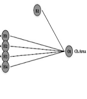
Figure 1 illustrates ANN (8: 4: 1) for modeling of 2, 5-HD analysis in urine samples. To determining the number of neurons in the hidden layer, different neural networks with different topologies were fitted to the data, and finally, the best neural network architecture was identified. It is noted that linear transfer function considered for the output layer, and Hyperbolic tangent is considered as a transfer function of the hidden layer. (Neural networks toolbox of Matlab 7.12.0).
 Trained for the Extraction Efficiency of 2, 5-hexandion")
Neural Network Architecture (3-4-1) Trained for the Extraction Efficiency of 2, 5-hexandion
4. Results and Discussion
2,5-HD extraction condition was optimized by the RSM. Therefore, three factors were optimized in this design. Table 2 shows the entire 48 runs. According to the quadratic model, the process response and three independent factors of empirical relationships are as follows:
The order of effectiveness of all model terms is as follows: C > A2 > A > B > B2 > C2 > AB > BC > AC (irrespective of the sign of model coefficients).
There was a coefficient of determination (R2) of 0.897. The R2 from the above quadratic equation was explained by independent variables of extraction temperature (A), extraction time (B), and sample volume (C).
| Run | Aa | Bb | Cc | Y (Observedd) | RSM Predicted | ANN Predicted | Run | A | B | C | Y (Observedd) | RSM Predicted | ANN Predicted |
|---|---|---|---|---|---|---|---|---|---|---|---|---|---|
| 1 | 80 | 5 | 15 | 182.45 | 116.002 | 137.81 | 25 | 60 | 5 | 10 | 433 | 421.507 | 436.04 |
| 2 | 80 | 10 | 15 | 130.65 | 192.078 | 123.15 | 26 | 60 | 10 | 10 | 483.48 | 478.926 | 486.86 |
| 3 | 80 | 20 | 15 | 297.7 | 295.217 | 291.74 | 27 | 60 | 20 | 10 | 652.17 | 543.752 | 659.71 |
| 4 | 80 | 30 | 15 | 291 | 333.006 | 298.02 | 28 | 60 | 30 | 10 | 640.03 | 545.228 | 626.96 |
| 5 | 70 | 5 | 15 | 104.95 | 183.687 | 122.99 | 29 | 50 | 5 | 10 | 165 | 293.277 | 187.41 |
| 6 | 70 | 10 | 15 | 153.33 | 249.171 | 147.69 | 30 | 50 | 10 | 10 | 202.7 | 340.14 | 194.85 |
| 7 | 70 | 20 | 15 | 324.25 | 331.127 | 329.03 | 31 | 50 | 20 | 10 | 217.23 | 384.747 | 212.87 |
| 8 | 70 | 30 | 15 | 315 | 347.733 | 357.96 | 32 | 50 | 30 | 10 | 210.67 | 364.039 | 209.55 |
| 9 | 60 | 5 | 15 | 69 | 156.729 | 151.46 | 33 | 80 | 5 | 5 | 600 | 591.332 | 584.9 |
| 10 | 60 | 10 | 15 | 117.17 | 211.621 | 131.42 | 34 | 80 | 10 | 5 | 638.3 | 672.461 | 639.3 |
| 11 | 60 | 20 | 15 | 286.13 | 272.393 | 280.94 | 35 | 80 | 20 | 5 | 787.23 | 785.706 | 803.04 |
| 12 | 60 | 30 | 15 | 297 | 267.817 | 293.19 | 36 | 80 | 30 | 5 | 756.68 | 833.602 | 754.81 |
| 13 | 50 | 5 | 15 | 65.23 | 35.127 | 152.18 | 37 | 70 | 5 | 5 | 612.7 | 645.761 | 602.95 |
| 14 | 50 | 10 | 15 | 95.2 | 79.428 | 117.23 | 38 | 70 | 10 | 5 | 654.3 | 716.298 | 659.61 |
| 15 | 50 | 20 | 15 | 107.25 | 119.017 | 113.75 | 39 | 70 | 20 | 5 | 818.5 | 858.36 | 822.83 |
| 16 | 50 | 30 | 15 | 147.1 | 93.256 | 73.32 | 40 | 70 | 30 | 5 | 797.2 | 835.073 | 763.12 |
| 17 | 80 | 5 | 10 | 449.7 | 394.036 | 415.26 | 41 | 60 | 5 | 5 | 578.8 | 605.536 | 582.35 |
| 18 | 80 | 10 | 10 | 496.7 | 472.639 | 491.69 | 42 | 60 | 10 | 5 | 618.2 | 665.492 | 620.67 |
| 19 | 80 | 20 | 10 | 662.5 | 580.831 | 666.45 | 43 | 60 | 20 | 5 | 778.1 | 736.371 | 770.28 |
| 20 | 80 | 30 | 10 | 649.7 | 623.674 | 644.75 | 44 | 60 | 30 | 5 | 751.3 | 741.9 | 720.44 |
| 21 | 70 | 5 | 10 | 502.03 | 455.094 | 439.01 | 45 | 50 | 5 | 5 | 565.3 | 470.688 | 547.75 |
| 22 | 70 | 10 | 10 | 545.6 | 523.105 | 520.98 | 46 | 50 | 10 | 5 | 586.9 | 520.042 | 586.58 |
| 23 | 70 | 20 | 10 | 694.8 | 610.114 | 678.5 | 47 | 50 | 20 | 5 | 611.73 | 569.737 | 601.16 |
| 24 | 70 | 30 | 10 | 658.53 | 631.773 | 660.28 | 48 | 50 | 30 | 5 | 597.2 | 554.083 | 602.64 |
The Coded Historical Design of Independent Factors and Their Corresponding Experimental Values, the RSM Model Predicted and ANN Model Predicted Values of Chromatography Area
The results of the ANOVA are shown in Table 3. All the independent variables were significant (P < 0.05). The F values and P values represent the high significance of the model and no significant lack-of-fit. The variables were not significantly correlated with each other (P > 0.05). The predicted values matched well with the experimental values (R2 = 0.9325 and Adj. R2 = 0.9165).
| Parameters | Statistics | ||||
|---|---|---|---|---|---|
| Sum of squares | Degree of freedom | Mean square | F Value | P Value | |
| Model | 2.576×10⁶ | 9 | 2.862×10⁵ | 58.30 | < 0.0001 |
| A | 2.346×10⁵ | 1 | 2.346×10⁵ | 47.79 | < 0.0001 |
| B | 2.121×10⁵ | 1 | 2.121×10⁵ | 43.20 | < 0.0001 |
| C | 1.886×10⁶ | 1 | 1.886×10⁶ | 384.27 | < 0.0001 |
| AB | 18872.33 | 1 | 18872.33 | 3.84 | 0.0573 |
| AC | 106.04 | 1 | 106.04 | 0.022 | 0.8839 |
| BC | 2134.46 | 1 | 2134.46 | 0.43 | 0.5136 |
| A2 | 1.273×10⁵ | 1 | 1.273×10⁵ | 25.92 | < 0.0001 |
| B2 | 33066.55 | 1 | 33066.55 | 6.74 | 0.0134 |
| C2 | 29815.63 | 1 | 29815.63 | 6.07 | 0.0184 |
| Residuals | 1.865×10⁵ | 38 | |||
| Cor Total | 2.762×10⁶ | 47 | |||
As presented in Figure 2A, the residuals are normally distributed and show a random scatter. Also, there is a linear correlation between predicted and actual response values that indicates a sufficient agreement between real data and model data (Figure 2B). These plots show that the model fits well to optimize the independent variables for the chromatography area prediction.
The model describes the entire experimental range of the study. It shows the comparison of the graphical representation of actual versus predicted values (Figure 2). The results of ANOVA of the linear model for the analysis of 2, 5-HD in urine samples are shown in Table 3.
The model came up with an F value of 69.90 and a P value of < 0.0001. P values of less than 0.05 were considered significant. According to the results, all factors were found to be highly significant (P < 0.05). According to the non-significant lack-of-fit, the model shows good predictability.

Comparison of graphical representation of actual versus predicted values
The predicted values were found to match well with the experimental values (R2 = 0.9325). The R2 value was in a reasonable agreement with Adj. R2 (Adj. R2=0.9165), which indicates fair predictability of the model.
The lowest training and verification errors in architecture 3-4-1 of an MLP neural network were permissible. According to the results, it was a suitable network for the prediction of optimization for the analysis of 2, 5-HD in urine samples.
The predictive performance of ANN and RSM models are presented in Table 4. The results showed that the ANN model in both tests and training sets had better performance in terms of R2 and RMSE compared to the RSM model. Smaller values of RMSE for ANN indicate less prediction error for this model. Considering the perfect prediction line, the predictions of the ANN model were closer than those of RSM models. Therefore, in terms of generalization capacity, the ANN model had more generalizability than the RSM model. Also, The ANN had a higher predictive accuracy, which might be related to its general ability to estimate the system nonlinearity. The RSM limitation is in a second-order polynomial.
| Measure | Neural Networks | RSM | ||
|---|---|---|---|---|
| Train | Test | Train | Test | |
| RMSE | 9.00 | 38.79 | 71.88 | 65.74 |
| R2 | 0.999 | 0.992 | 0.953 | 0.961 |
Comparison Between RSM and ANN
A large number of iterative calculations are required in the ANN model. In contrast, there is a single- step calculation for the response surface model
The most important limitation of the RSM method is that the experimental data are fitted to a polynomial model at the second order, while in practice using a second-order polynomial model is not compatible with all systems. In comparison, although the neural network model is a black box in nature, it can take into account the complexities of systems well, even with the limited number of experiments.
5. Conclusions
In this study, the main factors, extraction temperature (A), extraction time (B), and sample volume (C), were found to be highly significant (P < 0.05). The non-significant lack-of-fit showed good predictability. The ANN and RSM models were the same in predicted values. The results showed that the ANN method is preferable for recording nonlinear behavior and prediction. It had more generalizability, cost, and calculation time than the RSM model. Because of the ANN general ability to approximate the system nonlinearity, it had higher predictive accuracy. Unlike the response surface model, a large number of iterative calculations is required in the ANN model.
