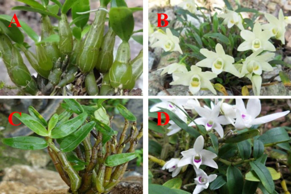
Materials
A total of 210 samples, including 10 original DHS samples, 10 original DHN, and 190 adulterated DHS samples with the known adulteration levels, were prepared in laboratory conditions as explained in the following subsection.
Preparation of the synthetically adulterated DHS samples
All samples were cut into small pieces and freezing-dried at -50 C and then pulverized and passed through a 60-mesh sieve (particle size-0.2 mm) under laboratory conditions. The 190 adulterated samples were prepared by mixing DHN with pure intermediate ultrafine powder of DHS to final concentrations (w/w) of 5%, 10%, 15%, 20%, 25%, 30%, 35%, 40%, 45%, 50%, 55%, 60%, 65%, 70%, 75%, 80%, 85%, 90%, and 95%, with ten repetitions per level. Approximately 500 mg of each sample was prepared and kept at -20 C until the ATR-FTIR analysis.
The ATR-FTIR spectrum of all the samples were used to establish PLS models for the quantitative analysis of DHN in adulterated DHS sample.
Collection of FTIR spectra of DHS samples
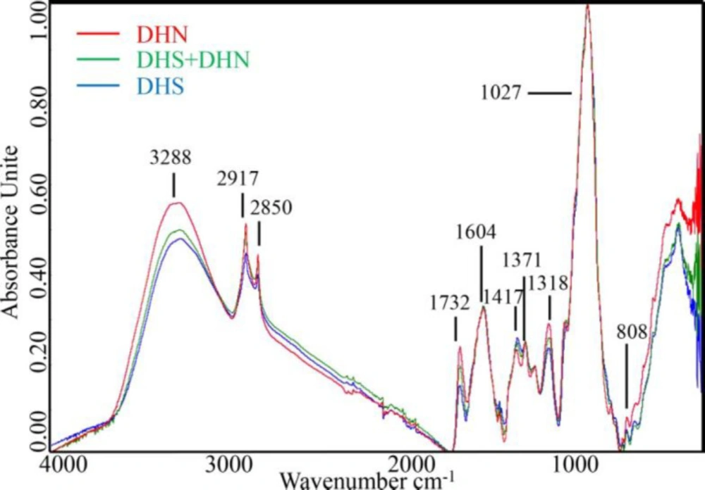
The spectra of the samples were recorded in the MIR range of 400-4000 cm−1 with a resolution of 4 cm−1 using a Nicolet iS50 FTIR spectrometer equipped with a diamond single reflection ATR accessory equipped by a diamond as a device manager (Thermo Scientific, Waltham, MA, USA). Each spectrum was collected for 32 scans in the absorbance mode. The mean spectrum of triplicate measurements was used as the FTIR spectrum of each sample.
The software OMNIC version 8 and Thermofisher Quantity Analyst 8 (Thermo Fisher Scientific) were used for spectral acquisition and further analysis, respectively.
FTIR spectral pre-processing
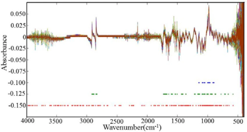
The spectral pre-processing is extremely important to reduce the interference and undesirable information and improve the contribution of chemical gradients. In this paper, different data pre-processing techniques including MSC, SNV, the first derivative and the second derivative by the Savitzky-Golay algorithm (15 data points), and the combinations of MSC with the first derivative, the SNV with the first derivative, MSC with the second derivative, and the SNV with the second derivative, were investigated to get reliable, accurate and stable models, because the background information and noise among the sample information are involved in the raw FTIR spectra . Then the results of eight different signal pretreatment methods were evaluated and compared.
Samples division method
The TQ-analyst 8 selection of training and test samples separately in classes. Thus, the samples were split into 105 (10 DHS samples, 95 DHS samples adulterated with DHN) for the training subset and 105 (10 DHS samples, 95 DHS samples adulterated with DHN) for the test subset.
Wavenumber selection method
Three different wavelength selection methods involving moving window partial least squares (MW-PLS), Monte carlo-uninformative variable elimination (MC-UVE), and interval random frog (iRF) were compared to obtain the effective wavelengths for the establishing of PLS models.
MW-PLS
As a wavenumber interval selection method, MW-PLS could make the PLS calibration model stable and avoid interference from the factors of irrelevant constituents (13). In this paper, the favourable spectral interval of the samples was chosen by the lowest Root Mean Square Error of Cross Validation (RMSECV), which could be calculated as following Equation 1.
Equation 1.
where yreal is the actual value of the investigated sample, ypre is the predicted value of the investigated sample. Generally, the lower RMSECV represents more information of the selected wavenumbers.
MC-UVE
Applying the MC-UVE, calibration samples are chosen arbitrarily to establish a chain of PLS models during each Monte Carlo (MC) sampling at first. Then the stability of each wave number is evaluated according to the PLS regression coefficient matrix during model calibration. To each MC procedure, the PLS regression coefficient is expressed as b = (b1, b2,…., bj…., bp). After M simulations, a PLS regression coefficient matrix B = (B1; B2;….BM) can be acquired. Since each bj represents the contribution of the j-th wave number to the PLS model, the stability of each wavenumber can be calculated by Equation 2.
Equation 2.
where mean (bj) and std (bj) are the mean and standard deviation values of the regression coefficient at j-th wave number in the PLS model.
According to the stability of all the wavenumbers, the wavenumbers, the stability value of which below the cut-off values, will be deleted by the last classification performance.
iRF
iRF is a wavelength interval selection method that considers the continuity of spectra (
15). Applying iRF, spectra are first fractionated into sub-intervals of the whole spectra by a moving window of a fixed width, and thus it can gain all of the possible continuous spectral intervals. The adopting possibility of each variable after N iterations is computed. The frequency of the j-th variable, j = ( 1, 2,….,p) chosen in these N variable subclasses, is expressed as
Nj. The adopting possibility of each variable can be accounted by Equation 3.
Equation 3.
In this paper, the best intervals with the lowest RMSECV are chosen. The width of the interval was set to 20 due to 7467 full spectral points, and this resulted in 7467 intervals, and each interval obtained 20 variables.
Quantification models with PLS
Partial least square regression (PLS) is one of the most common regression algorithms in chemometrics in general, particularly for spectroscopy.
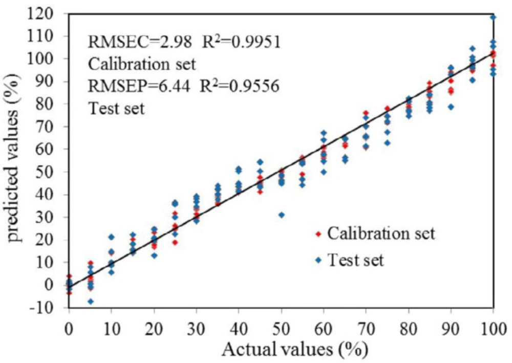
The PLS models were evaluated by leave-one-out cross-validation by mapping the number of factors against the RMSECV. The performance of the PLS models was commonly evaluated by the determined coefficients (R
2) and RMSECV. In addition, the root-mean- square error (RMSE), which respectively expressed as root-mean-square error of calibration (RMSEC) for calibration set and as root-mean-square error of prediction (RMSEP) for test set in this experiment, was used to appraise the established PLS model. A superior model should show high R
2 values while low RMSECV, RMSEC, and RMSEP (
2).