
1. Background
Acinetobacter has more than 50 types, most of which are environmental and non-pathogenic. Acinetobacter baumannii is an opportunistic pathogen that can cause both community-acquired and nosocomial infections, especially in intensive care unit patients (1). Most nosocomial infection transmission occurs through direct contact with hospital staff and equipment, highlighting the importance of factors such as proper disinfection of medical equipment, personnel awareness of infection risks, and the type of disinfectant agents used (e.g., biocides). Until three decades ago, A. baumannii infections were effectively treated with conventional antibiotics, but recently, due to the emergence of multidrug-resistant (MDR) strains, treatment of these infections has become challenging. According to reports from the World Health Organization (WHO), A. baumannii is one of the most serious organisms that evade the antibacterial effects of medicines through different mechanisms, such as efflux pumps and enzymatic degradation of drugs (2). The multidrug resistance of A. baumannii creates additional costs and pressure by prolonging the hospitalization period and has become a challenge for health systems worldwide, including in Iran. Another concern is the high resistance of A. baumannii to biocides. If high resistance of a type of bacteria to biocides becomes prevalent and coexists with antibacterial resistance, it can contribute to the development of new resistant microorganisms in that or other bacterial families through the transfer of resistant genes.
Controlling antimicrobial resistance (AMR) of A. baumannii, in addition to re-evaluating the effectiveness of common antimicrobial agents (such as antibiotics or biocides), requires investigating different characteristics of the source of A. baumannii (patient characteristics, environmental parameters, etc.) (3-5). One main problem in the treatment of bacteria-caused infections is the lengthy routine procedures for identifying the bacteria type or the expensive, time-consuming, and complicated polymerase chain reaction (PCR) tests that are rarely employed in clinics. Compared with traditional and PCR tests, AI-based approaches are not only time-saving and cost-effective but also facilitate practical research in the microbiology field (6). Past studies have shown that in the absence of traditional clinical techniques and instruments for distinguishing types of bacteria, AI can recognize the type of bacteria with a fast and automatic mathematical procedure (7). Recently, AI has demonstrated its significance in identifying and controlling AMR (8). Artificial neural networks (ANNs), as a type of AI algorithm, have shown reasonable performance in predicting the minimum inhibitory concentration (MIC) of antimicrobial peptides (AMPs) against A. baumannii isolates, even with limited data (9). This can be attributed to the robust capability of ANNs models in capturing complex non-linear patterns and thereby presenting better performance.
In many emergency medical cases where medical staff does not have enough time to wait for bacterial culture analysis to timely treat the bacterial infection of a patient, ANNs can be a useful tool for reducing the required time to prescribe antimicrobial agents, improving diagnostic and treatment accuracy, and decreasing the cost of medication. The ANNs models can support physicians in making the decision process more accurate and easier (10, 11). In other words, the application of ANNs models can be a basis for developing new strategies aimed at controlling infections. This model can contribute to the identification of potential antimicrobial molecules, accelerate the identification of AMR class, and optimize antibiotic compositions. Several past studies have used AI in the context of antibiotic resistance (10, 12). However, studies applying ANNs for classifying the AMR of A. baumannii isolates collected from patients in hospital wards (e.g., clinical isolates) and for predicting effective biocide doses to disinfect isolates from hospital environments (e.g., environmental isolates) are limited. It should be noted that the ANNs model was selected for this study framework considering features such as the nature of the data, dataset size, model complexity, and computational efficiency.
2. Objectives
The present study aimed to investigate whether artificial intelligence (AI) can improve the detection of AMR A. baumannii isolates in experimental conditions.
3. Methods
3.1. Bacterial Isolation Procedures
The initial step in implementing AI approaches, such as ANNs models, involves the collection and preparation of the necessary dataset. In this study, 103 clinical and 73 environmental isolates were collected from hospitalized patients and various locations across seven hospitals in Golestan province, northern Iran, over a one-year period (2021 - 2022). The samples were selected randomly using the convenience sampling method. The sample size was determined at a 95% confidence level using the following formula, where P1 represents the number of samples suspected of infection or pollution, and P2 denotes the number of samples with a positive test (α = 0.05, β = 0.10) (Equation 1):
Wound and burn specimens were collected by trained nursing personnel using a sterile wet cotton swab or a 3 mm punch weighing 0.03 grams. Respiratory and spinal fluid samples were obtained by a specialist physician and transferred to the laboratory. Environmental samples were collected at ambient temperature using sterile swabs from surfaces such as park tables, swimming pools, wheelchairs (4 × 4), and soil. Subsequently, the samples were homogenized using a homogenizer (BioMaster-Stomacher, Seward, England), and 0.1 cc of the resulting suspension was cultured on CHROMagar Acinetobacter (CMA, Sigma-Aldrich, USA).
Following phenotypic tests based on standard microbiological and biochemical methods (4), molecular identification and final confirmation of A. baumannii isolates were performed. Genomic DNA was extracted using the boiling method, and PCR was conducted to identify the blaOXA-51 gene using forward and reverse primers: F: 5'-TAATGCTTTGATCGGCCTTG-3' and R: 5'-TGGATTGCACTTCATCTTGG-3' (13, 14). After DNA extraction, it was crucial to ensure the absence of contamination by proteins or organic solvents. Once DNA purity was confirmed, a Control Mix, including primers and a probe, was added to the reaction mix before amplification. The PCR reaction was carried out in a final volume of 25 µL, consisting of 1 µL DNA sample, 1 µL of each primer, 12 µL of 2X Master Mix (containing 20 μM dNTP and 1.5 μM MgCl2), and 11 µL of distilled water. The reaction was performed in a thermocycler (Eppendorf, Germany) with the following cycling conditions: Initial denaturation at 94°C for 5 minutes, followed by 30 cycles of denaturation at 94°C for 60 seconds, annealing at 55°C for 1 minute, extension at 72°C for 1 minute, and a final extension at 72°C for 10 minutes. The resulting PCR products were then electrophoresed on a 1.5% agarose gel. The detection of 353 bp fragments confirmed the presence of isolates (Figure 1). Pseudomonas aeruginosa ATCC 27853 was considered as negative control and A. baumannii ATCC 19606 as positive control.
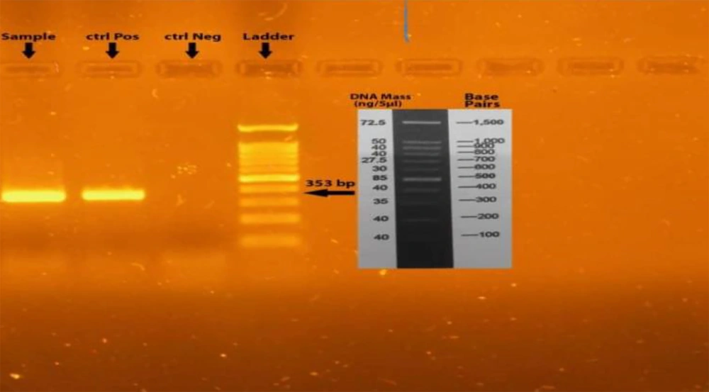
Figure 1.
Polymerase chain reaction (PCR) amplification of the blaOXA-51 gene
Clinical characteristics, including age, gender, sample source (e.g., burn wound, spinal fluid, sputum, lung secretions, urine, tissue biopsy), hospital sampling department (e.g., ICU, infectious, neurology, obstetrics, and gynecology), and the type of antibiotic used, were collected. Environmental characteristics included the antimicrobial agent used (biocide/antibiotic), sampling location (e.g., park table, yard soil, yard pool, wheelchair), material of the sample environment (e.g., metal, plastic, concrete, rubber, soil, water), infection contact risk (i.e., high to very high, moderate to high, low to moderate), and sampling season (i.e., summer, fall, winter, spring).
To determine the minimum inhibitory concentrations (MICs) of antibiotics — ciprofloxacin (CIP5), cefepime (FEP30), meropenem (MEM10), ticarcillin-clavulanic acid (TCC75 + 10), colistin (CS50), amikacin (AN30), doxycycline (DO30), gemifloxacin (GEM5), trimethoprim sulfamethoxazole (SXT1.25 + 23.75), ticarcillin (TIC75) — and biocides — benzalkonium chloride (BZK), benzethonium chloride (BZT), and chlorhexidine digluconate (CLX) — the broth microdilution method was used according to the CLSI-2021 standard tables guide (15). In brief, initial stock and two-fold serial dilutions of antibiotics and biocides were prepared, and 100 μL was inoculated into each well. The antibacterial effect of antimicrobials on the growth of all A. baumannii isolates after 24 hours was determined using optical density (OD560) and a final concentration of 106 - 107 CFU/mL. Pseudomonas aeruginosa ATCC27853 and Escherichia coli ATCC 25922 were used as controls for the susceptibility tests.
Clinical variables were assumed as input features of isolates, and the AMR class (i.e., R, I, S) of each isolate according to the MIC was considered the target value in the dataset. Similarly, environmental variables were assumed as input features, and the MIC class (i.e., H, M, L) was considered the target value. Since sampling locations had various access conditions for patients, medical staff, and hospital visitors, the qualitative parameter of infection contact risk was defined with respect to the number of people using the place within the sampling time slot. The weight of hospital visitors was considered as 1, while the weight of medical staff and patients was considered as 2 and 3, respectively. The weighted average was extracted, and if it was 2 or greater, the infection contact risk was assumed to be high to very high; if it was between 1.5 and 2, the risk was assumed to be moderate to high; and if it was between 1 and 1.5, the risk was assumed to be low to moderate. This procedure was repeated on three different days, and the average value of these days was used to determine the infection contact risk. Among the 30 environmental isolates, 50% had a high to very high infection contact risk, while 36.7% and 13.3% had moderate to high and low to moderate contact risks, respectively.
In the input features, only age and hospitalization period had a numeric nature, while others were categorical. With this data arrangement, there were six input and one output column for the ANNs model developed for both clinical and environmental datasets. Among the collected clinical isolates, the majority belonged to females, with 17 isolates (57%), and considering age, the majority belonged to the over 60 years old group, with 14 isolates (46.5%). Regarding the sample source and hospital sampling ward, most isolates belonged to the infectious and burn wound departments, with 63.5% and 33.5%, respectively. As for environmental isolates, the majority were extracted from park tables, with 16 (53.5%) samples, and most of these isolates were collected in spring, with 11 (36.5%) samples. Table 1 shows details of the input data features used for developing the ANNs model in this study.
Table 1.
Details of Used Data for Building Artificial Neural Networks Model for Clinical and Environmental Isolates
| Names | Value Ranges |
|---|---|
| Input features a | |
| Sex | 0, 1 means male, female |
| Age (y) | 31 - 78 |
| Sample source | Burn wound, spinal fluid, sputum, pulmonary secretions, urine, tissue biopsy |
| Sampling place | ICU, infectious department , neurology, obstetrics and gynecology |
| Hospitalization period (d) | 2 - 13 |
| Antibiotic name | CIP5, FEP30, MEM10, ticarcilin-clavunic acid, CS50, AN30, doxcycycline, GEM5, trimethoprim sulfametha xazole, tikarcilin |
| Target variables a | |
| Response to antibiotic | 3 categories: R, I, S (resistant, intermediate, sensitive) |
| Input features b | |
| Name of biocide | BZK, BZT, CLX, CIP5, FEP30, MEM10, ticarcilin-clavunic acid, CS50, AN30, doxcycycline, GEM5, trimethoprim sulfametha xazole, tikarcilin |
| Category | Antibiotic, biocide |
| Sample source | Park table, yard soil, yard pool, wheelchair |
| Sample environment | Metal, plastic, concrete, rubber, soil, water |
| Infection contact risk | 2 = < high-very high; 1.5 = < moderate-high < 2; 1 = < low-moderate < 1.5 |
| Sampling season | Winter, fall, spring, summer |
| Target variables b | |
| Biocide/antibiotic dose | 3 categories: H, M, L (high, moderate, low) |
Abbreviations: CIP5, ciprofloxacin; FEP30, cefepime; MEM10, meropenem; CS50, colistin; AN30, amikacin; GEM5 gemifloxacin.
a Clinical isolates.
b Environmental isolates.
3.2. Developing Artificial Neural Networks Model
The ANNs are computational models inspired by the structure and function of biological neural networks in the human brain (16). They consist of interconnected nodes, or neurons, arranged in layers: An input layer, one or more hidden layers, and an output layer (17). Neurons receive input signals, apply an activation function to process them, and transmit the result to neurons in subsequent layers, as illustrated in Figure 2.
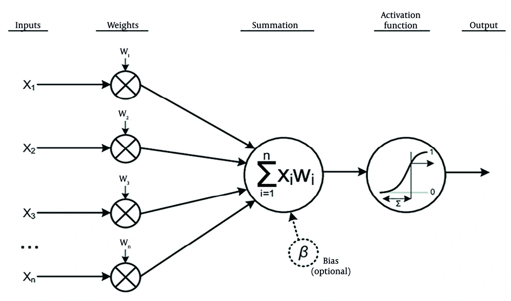
Figure 2.
Function of a single neuron in artificial neural networks (ANNs) model (18)
In ANNs, many such structures, as shown in Figure 2, can be interconnected to form layers. Consequently, the output of a neuron j in layer l is computed as follows (Equation 2):
- zj(l)is the weighted sum of inputs to neuron j in layer l.
- wij(l)is the weight of the connection between neuron i in layer l - 1 and neuron j in layer l.
- ai(l-1) is the output of neuron i in layer l -1.
- bj(l) is the bias term for neuron j in layer.
The output aj(l) of neuron j in layer l is obtained by applying an activation function f to the weighted sum of aj(l) = f (zj(l)). There are such common activation functions as Sigmoid, Hyperbolic tangent (tanh), Rectified Linear Unit (ReLU), and Softmax (19).
During training, the network learns by adjusting the weights and biases to minimize a predefined loss function, which measures the difference between the predicted output and the actual output of the data. The loss function is typically defined as the difference between the predicted output
With respect to the already arranged datasets corresponding to the categories of clinical and environmental isolates, where three distinct classes have been determined for each category, the ANNs model was developed to predict these three distinct classes. The ANNs model developed for the clinical dataset predicts the response class of various antibiotics (i.e., R, I and S) to these isolates according to their characteristics. Likewise, the implemented ANNs model for the environmental isolates dataset classifies the effective biocide dose into three classes (i.e., H, M, and L) to disinfect the isolates. Moreover, the first dataset comprises six features, while the second one encompasses seventeen features, which must be considered as the input layer of the ANNs models. The architecture of the ANNs models is akin to the conceptual framework illustrated in Figure 3.
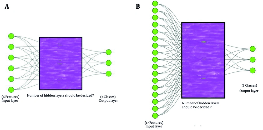
Figure 3.
Conceptual architecture of the artificial neural networks (ANNs) models for A, clinical isolates; and B, environmental isolates
Although environmental isolates initially comprised six input features, the corresponding conceptual ANNs model encompasses 17 features at the input layer, as shown in Figure 3. An empirical approach revealed that employing a traditional ANNs model with a six-neuron input layer yields inadequate accuracy scores, primarily due to all six features being categorical. Consequently, dummy variables were employed. A dummy variable, also referred to as an indicator variable, is a binary variable used mostly in statistical analysis to represent categorical data, taking the values 0 or 1 to signify the absence or presence of a particular category or characteristic. Dummy variables are instrumental in effectively incorporating categorical predictors into models (20). For instance, regarding the input feature of biocide name in the original environmental dataset, each of the 13 existing values was represented using a unique set of four-bit predictors. Hence, instead of a categorical feature for biocide name, a set of four new numerical features was introduced. This technique was applied to other categorical features of the environmental dataset, increasing the six categorical input features to 17 numeric features.
The determination of an optimal architecture for ANNs models is a critical aspect of developing predictive models in various domains. When designing an ANNs, researchers often face the challenge of balancing model complexity with performance. This necessitates careful consideration of the number of layers and neurons in each layer to ensure that the model effectively captures the underlying patterns in the data while avoiding overfitting (21). One approach for deciding on the architecture of an ANNs model is to commence with a simple structure and gradually increase complexity as needed. This iterative process involves experimentation with different configurations of layers and neurons in each layer while monitoring the model’s performance (22).
To calibrate the two ANNs models and determine their well-balanced architecture, a fine-tuning procedure was employed as a general approach, as follows:
- Defining metrics: Apart from several metrics such as accuracy, precision, recall, and F1-score, the primary metric considered was the accuracy of the models.
- Splitting the datasets: Each dataset was divided into two subsets: A training set and a test set. The training subset consists of 70% of the entire dataset, while the remaining 30% is used as the test set.
- Initializing model: In this step, the architectures of the models are defined, including the number of hidden layers, neurons per layer, and activation functions.
- Training the models: The training data is used to train the models. During training, the models learn to minimize the difference between their predictions and the actual target values.
- Evaluating performance of the models: Based on the chosen metric, which was accuracy, the models’ performance was assessed using the test subsets. The architecture or hyperparameters of the models should be adjusted according to the results as needed in an iterative manner.
- Finalizing the models: Once satisfied with the performance on the training and test subsets, the models can be considered final.
The calibration approach mentioned above was employed to determine the architecture of the ANNs in terms of the number of hidden layers and the number of neurons in each layer. Accordingly, Figure 4 illustrates the number of hidden layers versus the accuracy of ANNs models for both clinical and environmental isolates.
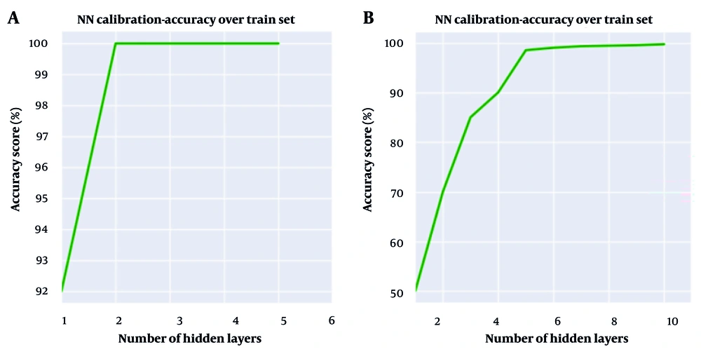
Figure 4.
Number of hidden layers versus accuracy score of artificial neural networks (ANNs) models during calibration process corresponding to A, environmental isolates; B, clinical isolates.
As shown in Figure 4A, two hidden layers represent the optimal point to achieve the best accuracy score for the ANNs model developed for environmental isolates, while the optimal number of hidden layers for the ANNs model for clinical isolates could be any number equal to or greater than five, based on Figure 4B. Although six hidden layers result in slightly better accuracy for clinical isolates, it was decided to use five hidden layers to reduce complexity and computation time without sacrificing significant accuracy.
The same approach was employed to determine the optimal number of neurons for each layer of both ANNs models. In this way, the number of utilized neurons in the first hidden layer of the developed ANNs model for environmental isolates was determined to be 34, as shown in Figure 5A. The same approach was employed for the second hidden layer, leading to the choice of eight neurons. Similarly, for the ANNs model of clinical isolates, the number of neurons utilized in each of the five hidden layers was determined. According to Figure 5B, the number 18 appeared to be a suitable choice for the number of neurons in the first hidden layer of this model. While selecting any number greater than 18 seems to yield a slightly more accurate result, the desire to avoid complexity in the model compelled us to opt for 18 as the optimal number of neurons in the first hidden layer. Following the same procedure described for the first hidden layer, the numbers 30, 18, 12, and 6 were identified as suitable numbers of neurons for the respective subsequent hidden layers.
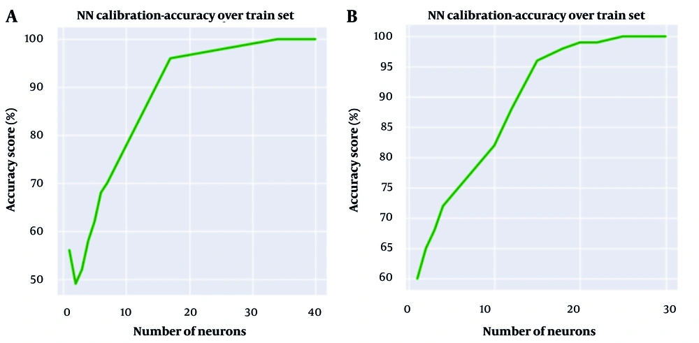
Figure 5.
Number of neurons in the first hidden layer versus accuracy score of developed Artificial neural networks (ANNs) models during the calibration process for A, environmental isolates; B, clinical isolates.
Figures 6 and 7 depict detailed versions of the conceptual ANNs models developed for environmental and clinical isolates, respectively, using the training dataset. As seen in Figure 6, the developed ANNs model for environmental isolates had two hidden layers, containing 34 and 8 neurons for the first and second hidden layers, respectively. In comparison, the ANNs model for antibiotics is more complex and consists of five hidden layers, encompassing 18, 30, 18, 12, and 6 neurons, consecutively. Table 2 summarizes the specifications of the software, libraries, operating system, and hardware used for implementing the ANNs model.
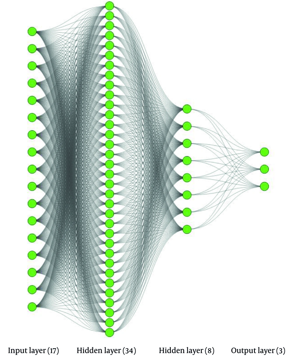
Figure 6.
The final architecture of artificial neural networks (ANNs) model developed for environmental isolates
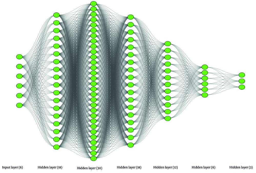
Figure 7.
The final architecture of artificial neural networks (ANNs) model developed for clinical isolates
Table 2.
Technical Details for Implementing Artificial Neural Networks Model Used in the Present Study
| Categories | Details |
|---|---|
| Software | Python (v3.9) |
| Libraries | TensorFlow (v2.4), Seaborn (v0.11.2), NumPy (v1.19), Pandas (v1.2), Matplotlib (v3.5.0), SKlearn (v1.1) |
| Operating system | Ubuntu 20.04 LTS |
| Hardware | NVIDIA GeForce RTX 3080, 16GB RAM, Intel Core i7 8th Gen Processor |
4. Results
In the experimental assay, 30 out of 103 clinical isolates (29% of clinical isolates) and 30 out of 73 environmental isolates (41% of environmental isolates) were identified as A. baumannii. In the clinical laboratory, the MIC of clinical isolates was obtained using 10 types of antibiotics to assess the level of AMR. Three classes of AMR — sensitive (S), intermediate (I), and resistant (R) — were determined based on the measured MIC and the interpretation criteria established by the producer company of the applied antibiotics. For environmental isolates, the MIC of BZK and BZT biocides was measured in the range of 1024 to 2 μg/mL, and three classes of MIC were determined similarly to the clinical isolates. These classes include high (H) for the highest MIC value of 512 μg/mL, moderate (M) for the second highest value of 256 μg/mL, and low (L) for values of 128 μg/mL or smaller. For CLX, values for H, M, and L classes were 1000, 500, and 250, respectively. In this way, 300 MIC data points for AMR of clinical isolates and 90 MIC data points for environmental isolates were set.
Because one of the main targets of this study was assessing the capability of ANNs for predicting the correct MIC class for isolates, while limited data of environmental isolates (90) was available using three types of biocides, antibiotics were also used on environmental isolates, thereby providing 300 additional MIC data points. When antibiotics were used as disinfecting agents for environmental isolates, MIC classes including S, I and R were renamed as L, M, and R classes as previously defined. Thus, the total number of MIC data points increased to 390 for environmental isolates.
During the laboratory tests, it was found that the minimum sensitivity level (R class of AMR) of clinical A. baumannii isolates was against CIP5 and TIC75, observed in 70% of isolates when both antibiotics were applied. Conversely, the maximum level of sensitivity (S class of AMR) was against CS50, observed in 60% of isolates, with the second maximum level of sensitivity against GEM5 and trimethoprim-sulfamethoxazole in 53.5% of isolates for both. Generally, 20% of clinical isolates showed the MDR phenotype, and 73.5% represented the extensively drug-resistant (XDR) phenotype (Figure 8).
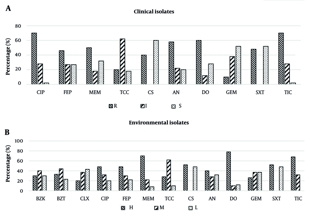
Figure 8.
Distribution of MIC values of antibiotics/biocides based on laboratory observations for A, clinical isolates; and B, environmental isolates.
Regarding the environmental isolates, the minimum sensitivity level (H class) was against DO30, observed in 76.5% of isolates. The maximum sensitivity level (L) was against CS50 and trimethoprim-sulfamethoxazole, observed in 47% of isolates when each of these antibiotics was employed. Additionally, the most effective biocide was CLX, with 43% of isolates requiring the L class of MIC. A total of 26.5% and 56.5% of environmental isolates showed MDR and XDR resistance phenotypes, respectively, against these two effective antibiotics (CS50 and trimethoprim-sulfamethoxazole). It was also observed that the most effective dose of BZK and BZT biocides against environmental isolates was 256 μg/mL, while it was 128 μg/mL for CLX. Figure 8 illustrates the distribution of MIC classes for different antibiotics and biocide/antibiotic applications to clinical and environmental isolates, respectively.
After model calibration over the training dataset of clinical and environmental isolates, the developed ANNs models were used on the test dataset. Considering the categorical nature of target data for MIC class of antibiotics/biocides (H, M, L) in the case of environmental isolates and AMR class of antibiotics (R, I, S) in the case of clinical isolates, the confusion matrix concept was employed to assess the accuracy of predictions (23). Figure 9 shows the confusion matrix over the test datasets. Concerning the response to antibiotics, Figure 9 reveals that 82 out of 90 predictions of AMR class by ANNs were correct, while it was 105 out of 117 for biocide/antibiotic MIC class. More specifically, Figure 8A shows that for I, R, and S classes of AMR, there are 20, 34, and 28 correct predictions, presenting 90% - 92% accuracy of predictions. Regarding the H, L, and M MIC classes for biocide/antibiotic dose, there are 46, 29, and 30 correct predictions, representing 87% - 97% accuracy. Thus, the error range of the applied ANNs models in the current study varies between 3% to 13%, which is similar to the error range of previously conducted studies (2% - 15%) using machine learning methods (24, 25). Generally, performance measures of the implemented ANNs model, such as precision, recall, F1-score, macro and micro-averaged F1, were better for the test dataset of clinical isolates. While the highest value of recall and F1-score were 0.93 and 0.92 for the S class of clinical isolates, in the case of environmental isolates, they were equal to 0.94 and 0.90 for the H class of environmental isolates.
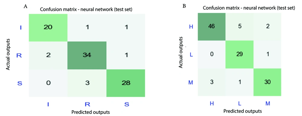
Figure 9.
Confusion matrixes for prediction of artificial neural networks (ANNs) model outputs for A, clinical isolates; B, environmental isolates.
5. Discussion
Acinetobacter is a major cause of nosocomial infections. In the present study, 29% and 41% of A. baumannii were isolated from clinical and environmental samples, respectively. According to a previous study in Iran, antibiotic resistance patterns among A. baumannii may vary widely in different parts of a country or from one country to another (4). In the present study, the minimum sensitivity level (R class of CIP5 and TIC75) was observed in 70% of clinical A. baumannii isolates. Biocides, as alternative antimicrobials, are widely used in hospitals and other health settings for disinfection of various medical devices and surfaces. However, the recent increase in the rate of microbial resistance to biocides has raised some concerns, and current principles have not been very successful in controlling nosocomial infections by MDR pathogens (3). In the current study, CLX had better potency compared to BZK and BZT biocides against environmental A. baumannii isolates, similar to previous studies’ reports (5, 26).
Today, AI algorithms are used for interpreting clinical microbiology data with associated gains in efficiency and diagnostic accuracy. Researchers have published a proof-of-principle study on the use of AI for automated interpretation of blood culture Gram stains and the use of AI in the clinical recognition of several common Gram stain morphologies (gram-negative rods, gram-positive cocci in clusters, and gram-positive cocci in chains) in positive blood culture smears (27, 28).
The best performance of the ANNs model in clinical isolates was for the R AMR class with 92% accuracy, indicating significant performance in recognizing resistant A. baumannii isolates. This can be helpful for medical staff to make better treatment decisions regarding the selection of the proper antibiotic type and dose for affected patients in each hospital ward. Among environmental isolates, the best performance of the ANNs model was for the L MIC class with 97% accuracy, implying a remarkable ability to detect isolates with a low required dose of biocides for disinfection. In contrast, the model’s accuracy was 87% in detecting environmental isolates with the H MIC class. This discrepancy can be attributed to the higher number of effective parameters on the MIC class of environmental isolates that were not considered, and hence the model could not clearly recognize their influence (e.g., level of exposure to UV, effect of prior infection and disinfection, etc.). However, the model can provide an initial proposal of the required MIC class for biocide and hence its dosage for disinfecting hospital areas exposed to infection.
The limitations of this study included a low number of isolates from each infection source, potential biases, and concerns regarding generalizability to other populations.
5.1. Conclusions
The following outcomes are obtained from the present work:
The application of the ANNs model, as a type of AI, can be a helpful approach for medical staff to facilitate and accelerate more accurate diagnoses, specifically in the context of new emerging threats to public health, such as the worldwide rising rate of AMR against A. baumannii. The ANNs model can predict the AMR class of various antibiotics for patients in hospitals and the MIC class of various biocides for disinfecting the hospital environment, taking into account a variety of affecting parameters with remarkable accuracy. Therefore, it can be a useful supporting tool for decision-makers in medical systems in hospitals due to its fast and simple application when there are limitations in resources such as time, budget, trained medical staff, and medical labs.
If a larger dataset can be used by increasing the number of samples for further development of this study, especially from hospitals located in different geographical locations worldwide, the model can be trained more precisely and comprehensively, and hence can represent more precise results (e.g., accuracy greater than 90%). In this way, this model can be practically used in hospitals as a part of treatment protocols, highlighting the benefits of cheap and fast diagnosis and prescription.