1. Background
Knee osteoarthritis, as one of the most common degenerative joint diseases, imposes a significant burden on healthcare systems and adversely affects patients’ quality of life. The assessment of disease severity is often based on the analysis of radiographic images and the Kellgren-Lawrence (KL) grading system, in which indicators such as joint space narrowing, osteophytes, and subchondral sclerosis are considered (1, 2). However, traditional methods based on expert visual assessment are limited by dependence on observer interpretation, inter-rater variability, and low sensitivity in detecting early disease stages (3). In recent years, machine learning algorithms have gained prominence in the automatic diagnosis of osteoarthritis severity and the accurate classification of KL grades (4, 5). One such advanced classifier is the Support Vector Machine (SVM) (6). The use of approaches that combine manual features — including local binary patterns (LBPs), Haralick features, gray-level co-occurrence matrix (GLCM), and discrete wavelet transform (DWT) — with features extracted from convolutional neural networks has improved detection accuracy and reduced classification errors (7, 8). Studies have shown that analysis of trabecular bone structure using fractal methods, such as directional fractal signature, can identify tissue changes associated with osteoarthritis even before clinical symptoms appear (3).
Additionally, the use of ensemble systems and rank-based models such as ordinal regression, along with advanced imaging techniques such as Gradient-weighted Class Activation Mapping (Grad-CAM), has enabled clinical interpretation of model decisions (1, 9). Furthermore, research has emphasized the role of clinical data — including age, gender, Body Mass Index (BMI), functional scores, and pain severity — in predicting the severity of osteoarthritis. Combining clinical data with imaging information in hybrid models has increased diagnostic accuracy, facilitated the identification of pathological subtypes of the disease, and improved the generalizability of models in clinical settings (10, 11). Recent randomized trials have explored various therapeutic modalities for knee osteoarthritis, including dextrose prolotherapy, high-intensity laser therapy (HILT), and instrument-assisted soft tissue mobilization (IASTM), each demonstrating promising effects on pain reduction and functional improvement (12-14). These findings underscore the importance of integrating diagnostic precision with evidence-based treatment strategies to optimize patient outcomes.
2. Objectives
Given the current gap in effectively integrating image and clinical features within an automated classification framework, the aim of this study is to develop a knee osteoarthritis diagnosis model based on image features extracted from radiographic images and the clinical characteristics of patients using the SVM algorithm. The novelty of this study lies in its integration of clinically interpretable structural features — such as the femoral-tibial axis angle, joint space width (JSW) ratio, subfemoral erosion, and osteophyte morphology — into a machine learning framework for automated knee osteoarthritis staging. Unlike prior studies that rely heavily on deep learning or abstract texture descriptors, our approach employs conventional image processing techniques and handcrafted features that are both transparent and clinically meaningful. The results of this study are expected to improve the accuracy of osteoarthritis severity classification and facilitate the design of automated clinical tools for early diagnosis and treatment decision-making.
3. Methods
This study utilized radiographic images from 44 patients (5 men, 39 women, aged 39 - 72 years) referred to the radiology department of Imam Ali Hospital in Bojnourd. The sample size (n = 44) was determined based on available clinical data and ethical limitations. This study was designed as an applied, retrospective, and observational research based on radiographic image analysis and clinical data.
Images were acquired using a SHIMADZU USISOL-40 digital device and retrieved via the MARCO PACS system in DICOM format, stored on CDs for processing to preserve image quality. All patients underwent clinical evaluation by an orthopedic specialist, with imaging performed in a standing position to capture the natural effect of body weight on knee joint space, which is critical for assessing joint space narrowing and osteoarthritis staging. Anteroposterior knee radiographs served as the primary data, with patients positioned to evenly distribute weight across both knees, enhancing clarity in joint space visualization. Lateral images, which were occasionally requested, were excluded from this study, consistent with methodologies in Yoon et al. (2).
Images were processed by isolating the left knee using the PACS software’s cropping tool. MATLAB (version 2013a) was employed for analysis. Initial image processing involved contrast adjustment to enhance bone structure visibility, followed by noise reduction using the Otsu thresholding algorithm to separate bone from background. The canny edge detection algorithm was applied to delineate bone edges based on brightness gradients, enabling precise feature extraction.
Four clinical features, aligned with the KL grading system and supported by prior studies, were extracted for osteoarthritis diagnosis (1, 3).
3.1. Femoral-Tibial Axis Angle
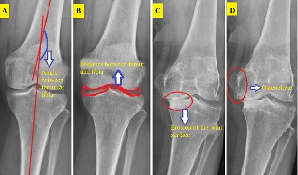
The femur and tibia curvature areas were segmented, and their centerlines drawn by connecting upper and lower points. The angle between these lines and the image horizon was calculated, with the difference (ranging from -8 to 8 degrees) indicating structural changes due to osteoarthritis (Figure 1). This was implemented in MATLAB as the TFA.M function.
3.2. Joint Space Width
The distance between femoral and tibial articular surfaces was measured in the middle knee region after cropping, contrast adjustment, and noise removal. The Otsu algorithm defined thresholds, and the Canny algorithm extracted horizontal joint space edges (Figure 1). Two vertical distances were measured, and their ratio (0 - 1) quantified joint space narrowing, implemented as JSW.M.
3.3. Subfemoral Bone Surface Erosion
A region between the femur and tibia was analyzed, with brightness intensity serving as an indicator of cartilage and bone erosion (Figure 1). Eroded areas, appearing brighter, yielded contrast values (100 - 250), normalized by dividing the standard deviation by the contrast to produce a 0 - 1 range, recorded as SCL2. M.
3.4. Osteophyte Detection
The knee joint was analyzed for bony outgrowths. A morphological gradient image highlighted vertical edges, and the Otsu method produced a binary image (Figure 1). The ratio of area to perimeter of prominent regions (initially 1 - 2) was normalized to 0 - 1 by subtracting one, saved as OST4. M.
All features were linearly normalized to a 0 - 1 scale to ensure uniform input for machine learning. Angular data were shifted and scaled, JSW features were preserved, erosion features were normalized via standard deviation ratios, and osteophyte features were linearly reduced.
A SVM with a “one-versus-the-rest” structure classified osteoarthritis stages (KL = 1 to KL = 4), with KL = 1 as the healthy reference due to ethical constraints on imaging healthy individuals. The SVM was chosen for its strong performance on small datasets, ability to model nonlinear relationships, and suitability for interpretable clinical classification tasks.
The dataset was split into training and test sets, with 10-fold cross-validation to assess model stability. Performance metrics included accuracy, sensitivity, specificity, and Cohen’s Kappa. Grid search optimized SVM parameters (kernel type, C penalty, etc.), with the radial basis function (RBF) kernel selected for its ability to handle nonlinear data boundaries. The LIBSVM MATLAB library facilitated implementation, with a cost-sensitive function to mitigate underfitting for underrepresented classes (e.g., KL = 4).
Feature weighting revealed the femoral-tibial angle as critical for advanced osteoarthritis stages, while joint erosion was key for early stages. Test data, excluded from training, were used to evaluate the final model, predicting KL stages and comparing them to physician diagnoses. The outcome variable was categorical, corresponding to KL grades (1 to 4), used for supervised classification.
Patient confidentiality was maintained by anonymizing DICOM images, excluding personal identifiers from the research database. Ethical considerations avoided unnecessary imaging of healthy individuals, aligning with clinical protocols.
4. Results
In this study, four clinical features related to knee osteoarthritis were extracted from knee radiographs: The angle between the femoral and tibial axes, the joint space distance, the amount of subarticular erosion, and the osteophyte assessment. To convert these clinical features into processable numerical values, image processing-based approaches were applied, and each feature was defined as a normalized scalar in the range [0,1].
4.1. Angle Between the Femoral and Tibial Axes
The angle difference between the centerlines of these two bones relative to the horizontal axis was calculated. In patients with severe osteoarthritis, the femoral axis is bent inward, and the angle difference is reduced compared to the normal position. This angle was extracted with high accuracy through Canny edge detection and Otsu thresholding, and its technical accuracy was consistent with clinical reality.
4.2. Joint Space Distance
The ratio of the left width to the right width was calculated by examining the lower region of the femur and the upper region of the tibia in the center of the joint. In patients with advanced osteoarthritis, this ratio tends toward zero, indicating bone adhesion on the medial side of the joint.
4.3. Subfemoral Erosion Feature
The brightness of the erosion area was determined by calculating the ratio of the standard deviation to the average contrast intensity. This index is usually reduced in osteoarthritis patients and indicates bone tissue degradation due to chronic pressure.
4.4. Osteophyte Feature
By creating a morphological gradient image and applying thresholding, bone growths were identified at the edges of the image. The area-to-perimeter ratio of these areas was defined as a geometric feature. Although this feature had limited clinical relevance in some cases, it performed well in diagnosing suspected cases without osteophytes.
The present study showed that each feature alone is able to relatively distinguish between different stages of the disease, and when combined, the recognition ability of the model increases significantly.
To evaluate the performance of the SVM model, k-fold cross-validation with k = 10 was used. In this method, the data were divided into 10 equal parts; in each iteration, one part was used for testing and 9 parts were used for training. Different kernels, including linear, polynomial, radial, RBF, and quadratic, and multilayer perceptron (MLP) were used for modeling, and the accuracy, sensitivity, and specificity for each case were reported as mean and standard deviation.
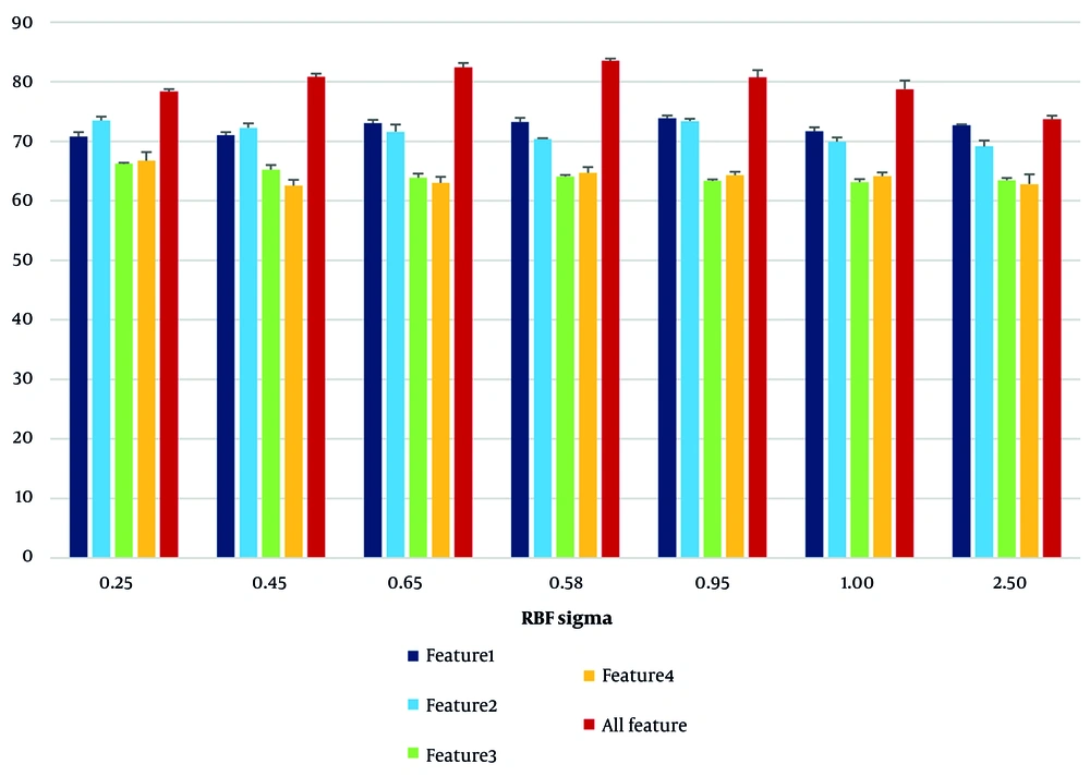
Initially, by changing the parameter σ in the RBF kernel, its effect on the accuracy of the model was investigated. The results in Table 1 show that the highest overall classification accuracy was achieved with a value of σ = 0.85 (83.53%), while at very small or larger values than the optimal limit, the accuracy decreased.
| RBF Sigma | Accuracy by First Features | Accuracy by Second Features | Accuracy by Third Features | Accuracy by Forth Features | Accuracy by All Features |
|---|---|---|---|---|---|
| 0.25 | 70.76 ± 0.77 | 73.46 ± 0.65 | 66.21 ± 0.19 | 66.74 ± 1.45 | 78.35 ± 0.40 |
| 0.45 | 71.01 ± 0.50 | 72.24 ± 0.77 | 65.21 ± 0.77 | 62.54 ± 0.96 | 80.78 ± 0.57 |
| 0.65 | 73.03 ± 0.54 | 71.58 ± 1.23 | 63.84 ± 0.70 | 63.01 ± 1.01 | 82.42 ± 0.72 |
| 0.85 | 73.24 ± 0.71 | 70.37 ± 0.13 | 64.04 ± 0.29 | 64.66 ± 0.97 | 83.53 ± 0.36 |
| 0.95 | 73.82 ± 0.49 | 73.37 ± 0.40 | 63.32 ± 0.28 | 64.29 ± 0.59 | 80.73 ± 1.21 |
| 1.00 | 71.65 ± 0.70 | 69.93 ± 0.70 | 63.12 ± 0.49 | 64.14 ± 0.62 | 78.74 ± 1.44 |
| 2.50 | 72.72 ± 0.13 | 69.11 ± 0.99 | 63.43 ± 0.37 | 62.80 ± 1.64 | 73.69 ± 0.61 |
a Values are expressed as mean ± SD.
b First feature: Angle between the femoral and tibial axes; second feature: Joint space distance; third feature: Subfemoral erosion feature; and forth feature: Osteophyte feature (expressed in percentage).
As can be seen in Figure 2, the effect of RBF sigma changes on the RBF kernel resulted in the model performance curve behaving nonlinearly with respect to σ changes, and the maximum accuracy was obtained at the midpoint. In addition, the performance analysis of each feature individually showed that the first feature (the angle between the femoral and tibial axes) performed best at σ = 0.95 with an accuracy of 73.82%, and the third feature (bone erosion) provided the lowest accuracy at most σ values.
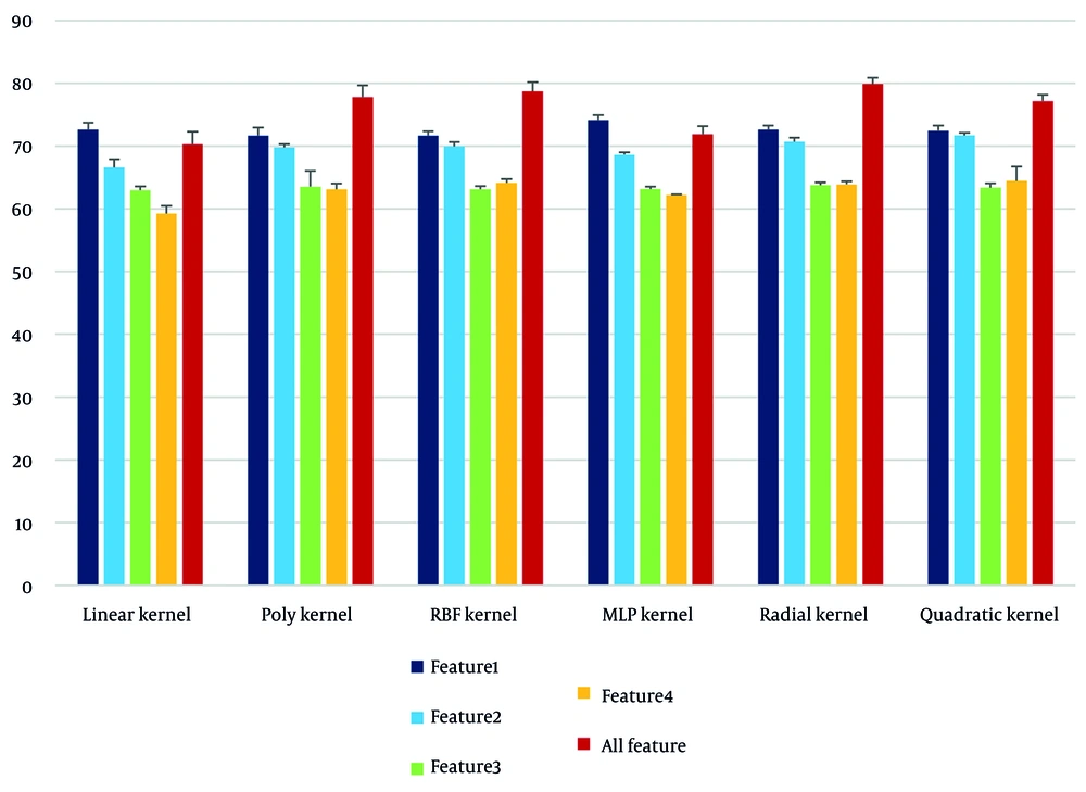
To investigate the effectiveness of different types of kernels in SVM modeling, a comparison was made between the results obtained by each kernel in the separation of each feature (Table 2). The following can be extracted from this table:
- The radial kernel demonstrated the highest performance among all kernels, with an overall accuracy of 79.89%.
- The linear kernel provided the lowest accuracy (70.29%) and performed particularly poorly for the fourth feature (osteophyte), with an accuracy of only 59.22%.
- The MLP had a high ability in the separation of the femur-tibia angle feature (74.14%), indicating the quasi-linear behavior of this feature in the feature space.
| Types of Kernels (or Models) | Accuracy by First Features | Accuracy by Second Features | Accuracy by Third Features | Accuracy by Forth Features | Accuracy by All Features |
|---|---|---|---|---|---|
| Linear | 72.61 ± 1.1 | 66.59 ± 1.32 | 62.97 ± 0.60 | 59.22 ± 1.25 | 70.29 ± 1.98 |
| Poly | 71.67 ± 1.28 | 69.81 ± 0.51 | 63.54 ± 2.49 | 63.11 ± 0.90 | 77.80 ± 1.86 |
| RBF | 71.65 ± 0.7 | 69.93 ± 0.70 | 63.12 ± 0.49 | 64.14 ± 0.62 | 78.74 ± 1.44 |
| MLP | 74.14 ± 0.82 | 68.62 ± 0.36 | 63.16 ± 0.39 | 62.18 ± 0.114 | 71.87 ± 1.29 |
| Radial | 72.61 ± 0.67 | 70.69 ± 0.66 | 63.77 ± 0.45 | 63.91 ± 0.49 | 79.89 ± 0.99 |
| Quadratic | 72.46 ± 0.83 | 71.70 ± 0.42 | 63.38 ± 0.67 | 64.42 ± 2.29 | 77.17 ± 1.01 |
Abbreviations: RBF, radial basis function; MLP, multilayer perceptron.
a Values are expressed as mean ± SD.
b First feature: Angle between the femoral and tibial axes; second feature: Joint space distance; third feature: Subfemoral erosion feature; and forth feature: Osteophyte feature (expressed in percentage).
This comparison is presented in Figure 3 as a bar chart that clearly shows the changes in the performance of the kernels for each feature and the full set of features.
The graph in Figure 3 shows that:
- The data related to the first feature exhibited stable and separable performance across different kernels.
- The third and fourth features require a model with high nonlinear resolution (such as the radial kernel) due to the dispersion in the feature space.
- Combining all features with the radial kernel, in addition to high accuracy, increased the sensitivity and specificity of the model.
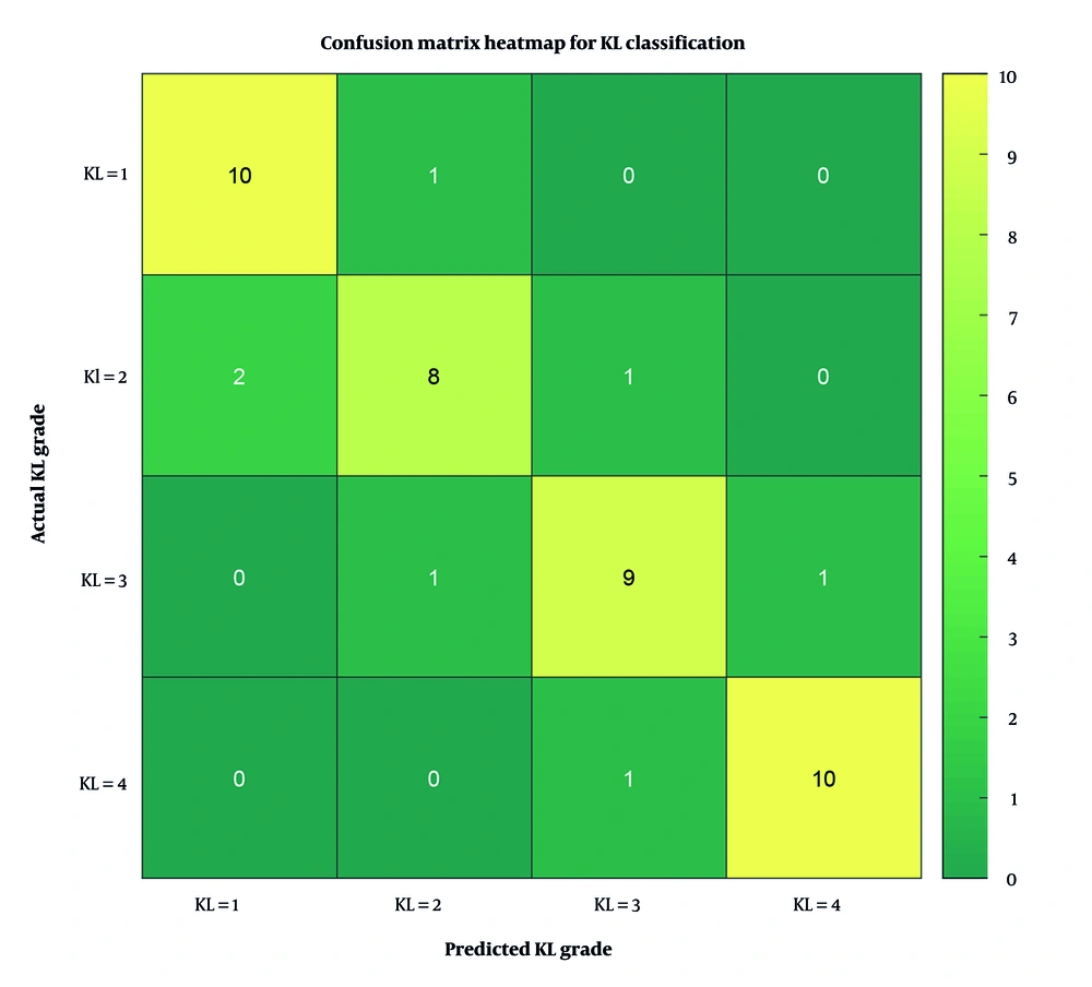
To further evaluate the model’s performance across individual KL grades, a confusion matrix was constructed and visualized as a heatmap (Figure 4). This matrix summarizes the number of correct and incorrect predictions for each class. As shown, the model achieved high accuracy in distinguishing KL = 1 and KL = 4 grades, while minor misclassifications occurred between adjacent grades such as KL = 2 and KL = 3.
Overall, these results indicate the success of combining clinical features and image processing in building an effective model for diagnosing the severity of knee osteoarthritis, and underscore the superiority of nonlinear kernels, especially radial, over other kernels in modeling complex medical data.
5. Discussion
The results of this study showed that the combination of clinical features extracted from knee radiographs and classification using the SVM algorithm can serve as an effective approach in assessing the severity of knee osteoarthritis. These findings are particularly significant from the perspective of medical physics, which focuses on bone structural parameters and imaging quality, as well as from the perspective of artificial intelligence, which analyzes data patterns and learns nonlinear relationships. Previous studies, such as those by Stachowiak et al., have emphasized the importance of trabecular bone texture and fractal analysis in the assessment of osteoarthritis (3); however, the present study, by focusing on structural-geometric features such as the angle between the axes of the bones and the joint distance, enables the extraction of features with high clinical interpretability. Furthermore, the use of conventional image processing algorithms, such as Otsu thresholding and Canny edge detection, has provided a feasible and low-cost processing pathway that can be readily implemented in clinical settings.
Analysis of the classification results with SVM showed that the first feature, the angle between the femoral and tibial axes, had high resolution (73.82% accuracy with σ RBF = 0.95 and 74.14% accuracy with MLP), indicating the mechanical role of this parameter in the progression of osteoarthritis. This finding is consistent with the studies of Yoon et al. and Khalid et al., who highlighted the role of bone axis deviation in predicting the need for therapeutic intervention, such as arthroplasty (2, 4). In contrast, features related to cartilage erosion and osteophytes, despite their clinical importance, performed poorly in classification alone (accuracy of about 63%), which may be attributed to the structural complexity of these phenomena in radiological images and their overlap with other features. The study by Tiulpin and Saarakkala also emphasizes that multivariate analysis of Osteoarthritis Research Society International (OARSI) features combined with KL grading may outperform single-feature models (1).
The use of different kernels in the SVM algorithm further demonstrated that nonlinear kernels, such as RBF and radial, outperform the linear kernel in classifying disease stages. The highest overall accuracy (79.89%) was achieved using the radial kernel and combining all features, indicating a nonlinear distribution of the data in the feature space. This is consistent with the findings of Ahmed et al. and Tariq et al., who have introduced the use of deep learning or hybrid (hybrid convolutional neural network plus MLP) models as effective methods for diagnosing osteoarthritis severity (9, 15).
The clinical relevance of accurate KL grade classification is further supported by recent interventional studies. For instance, Bayat et al. compared dextrose prolotherapy with corticosteroid injections and found superior mid-term functional outcomes with prolotherapy, emphasizing the importance of precise disease staging (12). Similarly, Taheri et al. demonstrated that HILT significantly improved pain and Western Ontario and McMaster Universities Osteoarthritis Index (WOMAC) scores, while Jafarsalehi et al. reported enhanced mobility and quality-of-life metrics following IASTM (13, 14). These studies highlight the therapeutic implications of accurate KL grading and reinforce the utility of automated classification systems in guiding treatment decisions.
One of the innovations of this study was the use of interpretable clinical features (angle, distance, erosion, osteophyte) along with controllable and easy-to-implement algorithms such as the SVM. Unlike deep models that require high processing resources, the proposed method can also be implemented in medical centers with limited equipment. In addition, the generalizability of the model was examined and confirmed through cross-validation (k-fold), which indicates the stability of the classifier’s performance against data changes.
One major limitation of this study is the relatively small sample size (n = 44), which may affect the generalizability of the model and increase the risk of overfitting. This constraint was due to limited access to ethically approved, high-quality radiographic data. To address this, we employed 10-fold cross-validation and selected low-dimensional, clinically interpretable features to reduce model complexity. Future studies with larger and more diverse datasets are essential to validate and extend the findings. Due to the limited sample size and categorical outcome, SHapley Additive exPlanations (SHAP) and receiver operating characteristic (ROC) analyses were not included. Future studies with larger datasets can incorporate these interpretability tools.
From an applied perspective, the results of this study can help in the development of computer-aided diagnosis (CAD) systems in imaging units. Rapid and automated analysis of radiographic images using a trained SVM model can play a role in patient classification, prioritization of therapeutic interventions, and even in planning joint replacement surgeries.
5.1. Conclusions
This study developed an automated classification model to assess knee osteoarthritis severity using radiographic image processing, focusing on four clinical features: Femoral-tibial axis angle, joint space distance, joint erosion rate, and osteophyte detection. A SVM algorithm with linear and nonlinear kernels was employed, with nonlinear kernels — particularly radial and RBF — demonstrating superior performance in distinguishing disease stages. The model achieved a peak accuracy of 79.89% when all features were combined with the radial kernel, highlighting the importance of feature integration and classifier selection. Notably, the model’s ability to analyze bone geometry, especially the femoral-tibial angle, was significant in predicting disease severity. Although the proposed model may offer practical advantages in resource-limited settings due to its simplicity and interpretability, further validation on larger, multi-center datasets is essential to confirm its generalizability and clinical applicability. Future research should incorporate multi-source data, including demographic characteristics and additional imaging modalities such as magnetic resonance imaging (MRI) and computed tomography (CT), to enhance diagnostic accuracy and develop multimodal intelligent systems.
