Pharmacophore modeling
Before beginning of pharmacophore modeling procedure, a total of 59 glucagon receptor antagonists were gathered from published resources. As mentioned before, of these molecules, 20 were selected to form a training set based on broad coverage of activity range and structural diversity using Kennard and Stone algorithm. The top ten hypotheses were composed of HYP, HYP aliphatic, HBA lipid, HBD, and PI features.
Table 2 reports the statistics of the generated pharmacophore hypotheses. The values of the ten hypotheses such as pharmacophore features, root-mean-square deviations (rmsd) correlation (r), cost values, and Fischer confidence levels showed statistical significance (
Table 2).
| Hypothesis | Total cost | Cost difference a | RMSD | Error cost | Correlation | Features b |
|---|
| 1 | 113.989 | 64.38 | 2.14865 | 93.5037 | 0.805377 | HBD, HYP, PI |
| 2 | 116.752 | 61.617 | 2.21863 | 96.5597 | 0.790605 | HBD, HYP aliphatic, PI |
| 3 | 120.691 | 57.678 | 2.31742 | 101.041 | 0.768374 | HBD, HYP aliphatic, PI |
| 4 | 124.388 | 53.981 | 2.40129 | 104.999 | 0.748323 | HBD, HYP aliphatic, PI |
| 5 | 124.527 | 53.842 | 2.26536 | 2.26536 | 0.786852 | HBA lipid, HBA lipid, HYP aliphatic |
| 6 | 125.362 | 53.007 | 2.4219 | 105.993 | 0.74324 | HBD, HYP , PI |
| 7 | 127.274 | 51.095 | 2.37537 | 103.761 | 0.758553 | HBA lipid, HBA lipid, HYP |
| 8 | 128.58 | 49.789 | 2.44362 | 107.05 | 0.739536 | HBD, HBD |
| 9 | 134.536 | 43.833 | 2.55966 | 112.855 | 0.707545 | HBA lipid, HYP aliphatic, PI |
| 10 | 134.67 | 43.699 | 2.58868 | 114.349 | 0.699263 | HBA lipid , HYP aliphatic, PI |
Cost difference = null cost - total cost.
Abbreviations used for features: hydrogen bond acceptor (HBA), hydrogen bond donor (HBD),hydrophobic (HYP), positive ionizable (PI)
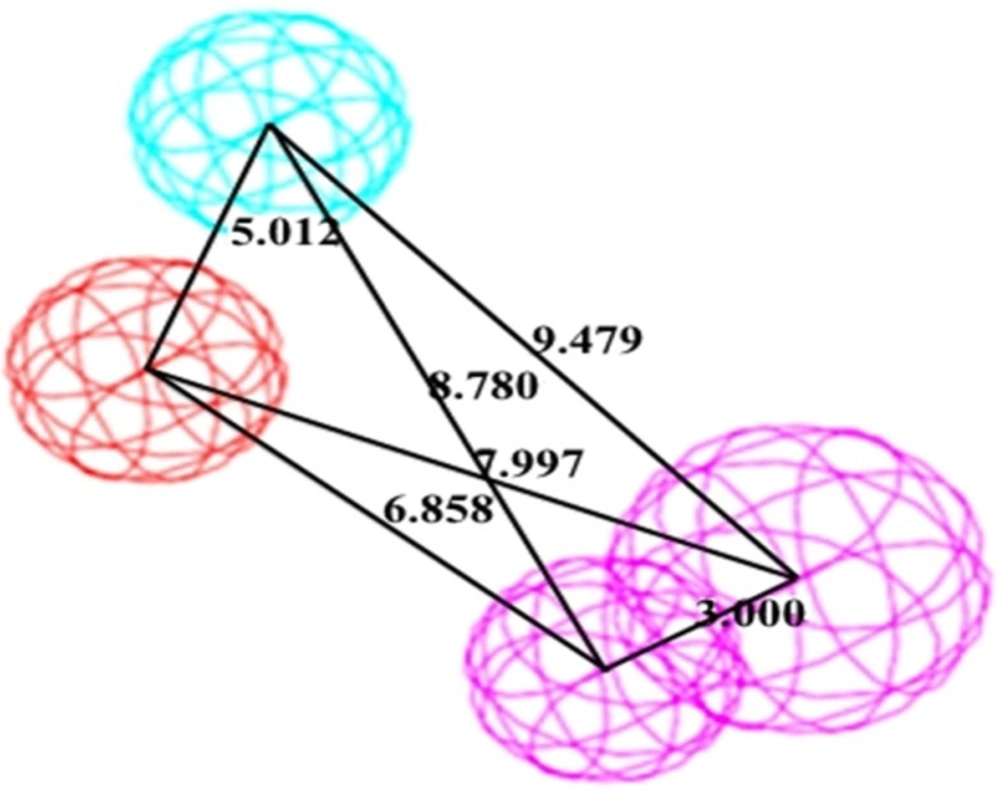
A significant pharmacophore model should have a large difference between its total and null cost values. In this work, the best hypothesis, Hypo1, as indicate in
Figure 1 and reported in
Table 2 is characterized by the lowest total cost value (113.989), the highest cost difference (64.38) and the lowest
RMSD (2.14865).The developed pharmacophore showed the highest correlation coefficient value of 0.80, highlighting its strong predictive ability. The fixed cost and null cost are 66.403 and 178.369 bits, respectively. The total cost is low and close to the fixed cost, as well as being less and differs greatly from the null cost. The entire evidences indicate that the developed model has good predictive ability. Consequently, Hypo1 was chosen as the best pharmacophore model for further analyses and application.
The best pharmacophore model Hypo1 represented with distance constraints. Pharmacophoric features colored as follows: PI (Red), HBD (Violate), hydrophobic (Blue)
Application of developed Pharmacophore model on training set
As mentioned above, all of the molecules in the studied dataset set were categorized into four different groups based on their biological activity (IC
50) values: active (IC
50 ≤ 0.5µM, ++++), moderately active (0.5 ≤ IC
50 ≤ 5µM, +++) less active (5 ≤ IC
50 ≤ 50, ++) and inactive (IC
50 > 50, +) (
Table 3). The activity of each training set molecule was predicted by a fitting procedure based on the best pharmacophore model, Hypo1, and the results are displayed in
Table 3. As it can be seen, three of training set molecules were predicted as having different IC50s than their experimental values. It must be noted that all active molecules in the training set were predicted as active glucagon receptor antagonists. One moderately active compound, molecule 19, was underestimated as a less active compound. Also, the estimated activity of two molecules, 16, and 17 were underestimated. Error values depict the ratio between the experimental and estimated activity values. Positive error values are calculated when the predicted activity value is higher than the observed value and a negative value shows the opposite. All of the active compounds listed in
Table 3 contained all of the five chemical features in Hypo 1, whereas all of the other compounds mapped four or less pharmacophoric features of hypothesis.
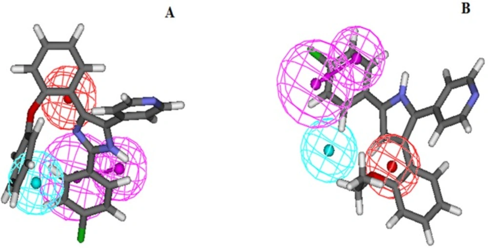
Figure. 2A and B depicts the mapping of the most and least active molecules (molecule 13 and 19 respectively) of the training set on Hypo1, respectively.
| Name | IC50
| Fit Value a | Error b | Activity scale c
|
|---|
| experimental | estimate | experimental | estimate |
|---|
| 1 | 0.07 | 0.064 | 7.36342 | -1.08746 | | |
| 2 | 0.08 | 0.068 | 7.33657 | -1.16831 | | |
| 3 | 0.1 | 0.071 | 7.32137 | -1.41017 | | |
| 4 | 0.3 | 0.092 | 7.2064 | -3.24652 | | |
| 5 | 0.05 | 0.096 | 7.18909 | +1.92327 | | |
| 6 | 0.12 | 0.135 | 7.0406 | +1.12802 | | |
| 7 | 0.34 | 0.156 | 6.97872 | -2.17819 | | |
| 8 | 0.05 | 0.163 | 6.95839 | 3.27144 | | |
| 9 | 0.1 | 0.164 | 6.95596 | +1.64491 | | |
| 10 | 0.26 | 0.191 | 6.89303 | -1.36742 | | |
| 11 | 0.117 | 0.202 | 6.8661 | +1.72909 | | |
| 12 | 0.3 | 0.232 | 6.80592 | -1.29105 | | |
| 13 | 0.29 | 0.271 | 6.73877 | -1.06922 | | |
| 14 | 1.4 | 0.811 | 6.263 | -1.72595 | | |
| 15 | 0.8 | 0.885 | 6.22506 | +1.1065 | | |
| 16 | 0.18 | 0.8852 | 6.22506 | +4.91778 | | |
| 17 | 0.16 | 0.920137 | 6.20825 | +5.75086 | | |
| 18 | 2.68 | 1.54629 | 5.98281 | -1.73318 | | |
| 19 | 14.2 | 1.81386 | 5.9135 | -7.82861 | | |
| 20 | 2.8 | 2.28485 | 5.81324 | -1.22546 | | |
Positive value indicates that the predicted IC50 is higher than the experimental IC50; negative value indicates that the predicted IC50 is lower than the experimental IC50.
Fit value indicates how well the features in the pharmacophore map the chemical features in the compound.
Activity scale: active,
(IC50 ≤ 0.5 µM); moderately active,
(0.5 < IC50 ≤ 5 µM); less active,
(5 < IC50 ≤ 50 µM); poor active,
(IC50 > 50 µM).
Overlay of most active (A) and least active (B) molecules in the training set upon the best pharmacophore model Hypo1. For details of Pharmacophoric features colors refer to Figure 1
Validation method
As well as the training set prediction by Hypo1, the predictive ability of the best developed pharmacophore model was tested using additional methods such as cost analysis, prediction of biological activity of test set, Fischer randomization, and E value calculation. Cost analysis is based on the statistical cost values generated during pharmacophore model building phase. A diverse test set was employed to verify if the pharmacophore model predicts the biological IC50 of the molecules that are structurally distinct to the training set. The Fischer randomization test was also used to verify that the chosen pharmacophore model was not generated as a result of chance correlation. The E value calculation was built to verify the selectivity of the developed pharmacophore model towards actives molecules rather than in-actives.
Cost analysis
The “common feature pharmacophore generation”algorithm generated three cost values during pharmacophore building step to evaluate the quality and reliability of the pharmacophore hypothesis. As described in Method section, the first cost value is the fixed cost value (also called ideal cost) denotes the simplest model that fits the data completely. The second one is the null cost value (no correlation cost) denotes the highest cost of a pharmacophore with no features estimating the activity to be the average IC
50s of the training set molecules. A statistical significant and predictive pharmacophore hypothesis should have a large difference between these two cost values. Hypo1 was generated with a fixed cost value of 66.403 and a null cost value of 178.369, thus with a difference of 64.38. The third cost is the total cost value estimated for every pharmacophore hyothesis and should be close to the fixed cost value. A large difference between the total and null costs shows a more predictive and statistical meaningful pharmacophore model. Hypo1 scored a total cost value of 113.989, which is closer to the fixed cost, for a cost difference of 134.158 (reported in
Table 2).
Test set prediction
A set of 39 molecules with structures quite similar to training set and range of IC
50 values was employed to assess the best developed pharmacophore model, Hypo1. The chemical structures of the test set compounds are provided in
Table 1. The “Ligand Pharmacophore Mapping”protocol implemented in ADS with the Best Flexible Search option was applied to map all of the molecules in test data (
Table 4). Using this protocol, the activity values were calculated for each molecule in test data. In particular, no compound in the test set was predicted with an error value more than 10, thus not exhibiting more than one order of magnitude between experimental and estimated activities (
Table 4). Noticeably, 76.92% (30 molecules) of the test set molecules were predicted within their IC50 scales while the remaining 23.07% (9 molecules) were estimated in different activity scales. From these 9 molecules, 3 active molecules were underestimated as active; 4 moderately active molecules were overestimated as active molecule and 2 less active molecules were overstimated as moderately active and active molecules. All of the less active and inactive compounds were predicted within their activity scales.
Fit values were calculated using all ten hypotheses and correlated with experimental activities. The best hypothesis, Hypo1, showed a correlation coefficient (R2 = 0.805).
| Name | IC50(µM)
| Error | Fit Value | Activity scale
|
|---|
| experimental | estimate | experimental | estimate |
|---|
| 21 | 0.19 | 0.059793 | -3.177619 | 7.39545 | ++++ | ++++ |
| 22 | 0.21 | 0.059814 | -3.510872 | 7.3953 | ++++ | ++++ |
| 23 | 0.59 | 0.05992 | -9.846429 | 7.39453 | +++ | ++++ |
| 24 | 0.09 | 0.060491 | -1.487815 | 7.39041 | ++++ | ++++ |
| 25 | 0.11 | 0.062979 | -1.746603 | 7.3729 | ++++ | ++++ |
| 26 | 0.1 | 0.065565 | -1.525216 | 7.35543 | ++++ | ++++ |
| 27 | 0.09 | 0.065565 | -1.372694 | 7.35543 | ++++ | ++++ |
| 28 | 0.15 | 0.06803 | -2.204903 | 7.3394 | ++++ | ++++ |
| 29 | 0.13 | 0.069603 | -1.867725 | 7.32947 | ++++ | ++++ |
| 30 | 0.053 | 0.072127 | +1.360883 | 7.314 | ++++ | ++++ |
| 31 | 0.023 | 0.072832 | +3.166617 | 7.30978 | ++++ | ++++ |
| 32 | 0.027 | 0.073341 | +2.716326 | 7.30675 | ++++ | ++++ |
| 33 | 0.06 | 0.0735 | +1.225003 | 7.30581 | ++++ | ++++ |
| 34 | 0.1 | 0.073576 | -1.359146 | 7.30537 | ++++ | ++++ |
| 35 | 0.1 | 0.07371 | -1.356675 | 7.30458 | ++++ | ++++ |
| 36 | 0.014 | 0.075042 | +5.360157 | 7.29679 | ++++ | ++++ |
| 37 | 0.08 | 0.075179 | -1.064134 | 7.29601 | ++++ | ++++ |
| 38 | 0.19 | 0.077713 | -2.444887 | 7.28161 | ++++ | ++++ |
| 39 | 0.15 | 0.078717 | -1.905558 | 7.27603 | ++++ | ++++ |
| 40 | 0.11 | 0.095641 | -1.150136 | 7.19146 | ++++ | ++++ |
| 41 | 0.13 | 0.107363 | -1.210845 | 7.14124 | ++++ | ++++ |
| 42 | 0.05 | 0.125811 | +2.51622 | 7.07238 | ++++ | ++++ |
| 43 | 0.02 | 0.160961 | +8.04805 | 6.96538 | ++++ | ++++ |
| 44 | 0.04 | 0.162512 | +4.0628 | 6.96121 | ++++ | ++++ |
| 45 | 1.44 | 0.386826 | -3.722604 | 6.58458 | +++ | ++++ |
| 46 | 0.95 | 0.429214 | -2.213348 | 6.53943 | +++ | ++++ |
| 47 | 0.14 | 0.477763 | +3.412593 | 6.49289 | ++++ | ++++ |
| 48 | 0.13 | 0.497664 | +3.828185 | 6.47516 | ++++ | ++++ |
| 49 | 0.074 | 0.5272 | +7.124324 | 6.45012 | ++++ | +++ |
| 50 | 1.15 | 0.568055 | -2.024452 | 6.41771 | +++ | +++ |
| 51 | 0.99 | 0.57235 | -1.729711 | 6.41444 | +++ | +++ |
| 52 | 0.42 | 0.577576 | +1.375181 | 6.41049 | ++++ | +++ |
| 53 | 1.69 | 0.579427 | -2.916675 | 6.4091 | +++ | +++ |
| 54 | 0.061 | 0.621097 | +10.18192 | 6.37894 | ++++ | ++ |
| 55 | 0.027 | 0.632999 | +23.44441 | 6.3707 | ++++ | ++ |
| 56 | 1.36 | 0.827474 | -1.643556 | 6.25435 | +++ | +++ |
| 57 | 0.18 | 0.8425 | +4.680556 | 6.24653 | ++++ | +++ |
| 58 | 2.8 | 0.903949 | -3.09752 | 6.21596 | +++ | +++ |
| 59 | 0.43 | 1.05557 | +2.454814 | 6.14861 | ++++ | +++ |
| 60 | 0.49 | 1.1109 | +2.267143 | 6.12642 | ++++ | +++ |
Fischer randomization test
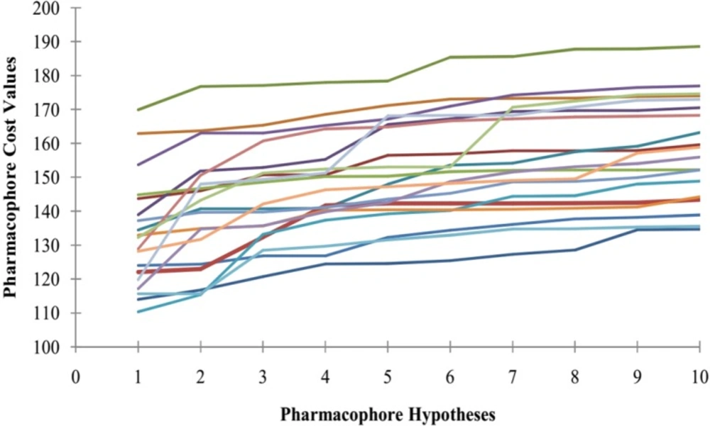
Furthermore, Fischer randomization test technique was applied to evaluate the statistical robustness of developed pharmacophore model (Hypo1). The third method to validate the robustness of the developed model is based on Fischerʹs randomization technique. The observed biological activities of the training set were shuffled randomly and the resulting training set was used in common feature pharmacophore generation protocol with the parameters selected for the original model building step. Thereby, a set of 19 random tables was generated to reach a 95% confidence level that the best pharmacophore, Hypo1, was not developed by chance.
Figure 3 indicates that none of the randomly developed pharmacophore models were generated with better statistical values than Hypo1. The results of Fischer randomization test technique clearly demonstrate that the original hypothesis is far more superior to those of the 19 randomization produced hypotheses, which give confidence on developed pharmacophore model.
The difference between cost values of developed pharmacophore model and the scrambled models
Estimation of Enrichment factor
The GH score has been effectively used to determine model selectivity (best model) accuracy of hits, and the recall of active molecules from a molecule dataset consisting of known active and inactive molecules. GH scoring methodology has been successfully applied for quantification of model selectivity and coverage of activity space from database mining (
57) and for the evaluation of the effectiveness of similarity search in databases containing both structural and biological activity data (
58). The GH score contains a coefficient to penalize excessive hit list size and, when evaluating hit lists, is calibrated by weighting the score with respect to the yield and coverage. The GH score ranges from 0, which indicates the null model, to 1, which indicates the ideal model (i.e., containing all of, and only, the active ligands). The GH value is expected to be greater than 0.7 (
59). It is considered a relevant metric, as it takes into account both the percent yield of actives in a database (%Y, recall) and the percent ratio of actives in the hit list (%A, precision). The GH scoring formula can be applied to identify best tolerance for an analysis testing different
RMS tolerance in fixed atomic position. For fixed positions tolerance an optimum GH score can be calculated. This method can also be applied to calculate highest GH score for the activity of a class of compounds clustered in a group. Hence, using the GH score method for each cluster of compounds aimed for particular activity, one can associate ownership for each cluster.
Generated pharmacophore model was also validated employing which determines whether the best hypothesis can choose active molecules during the virtual screening procedure from a database of 1733 molecules consisting of 39 experimentally determined glucagon receptor antagonists retrieved from the recently published studies.
Statistics used in this section includes calculation of false positives, false negatives, enrichment factor, and goodness of hit to determine the robustness of the generated hypotheses (
47) (reported in
Table 5). Not only should the pharmacophore model generated predict the biological activity of the molecules applied for model building, but it should also be skilled for predicting the biological activities of other molecules as active or inactive.
Using the best developed pharmacophore model, Hypo1, 35 molecules (Ht) were retrieved as hits from the database screening.
Among these hits, 32 (Ha) molecules were from the A list of known antagonists. Therefore, the enrichment factor was calculated to be 40.62, indicating that it is 40.62 times more probable to pick an active compound from the database than an inactive one. This value of enrichment factor and a GH score of 0.89 indicated the quality of the model and high efficiency of the screening test.
As it can be seen from this table, selected pharmacophore model is successful in retrieving 90% of the active molecules, 3 inactive molecules (false positives) and predicted 7 active molecules as inactive (false negatives).
| Serial No. | Parameters | Results |
|---|
| 1 | Total number of molecules in database (D) | 1733 |
| 2 | Total number of actives in database (A) | 39 |
| 3 | Total number of hit molecules from the hit database (Ht) | 35 |
| 4 | Total number of active molecules in hit list (Ha) | 32 |
| 5 | % Yield of actives (Ha/Ht) × 100 | 91.4 |
| 6 | % Ratio of actives (Ha/A) × 100 | 82.05 |
| 7 | Enrichment Factor (EF) | 40.62 |
| 8 | FALSE negative [A-Ha] | 7 |
| 9 | FALSE positives [Ht-Ha] | 3 |
| 10 | Goodness of hit (GH)* | 0.89 |
[(Ha/4HtA) (3A + Ht) × (1–(Ht –Ha) /(D–A))]
Virtual Screening and drug-likeness prediction
In drug design and discovery procedure virtual screening (database searching) is an efficient alternative way to high throughput screening (HTS). The best pharmacophore model, Hypo1, was used as a 3D query to search a chemical database, Maybridge for a total of 174000 compounds. The “Ligand Pharmacophore Mapping protocol”with the Best Flexible Search option was employed to search these databases. Inhibitory activity values were estimated for the compounds obtained from the database screening. A total of 2000 molecules were mapped upon all of the pharmacophoric features present in Hypo1. A total of 100 compounds mapped in previous step scored an estimated activity value less than 0.07 µM and were considered for further studies.
Lipinski’s rule of five evaluation
Drug-likeness properties are one of the key indicators for selecting the molecules for
in-vitro studies, which includes molecular or physicochemical properties that contribute to favorable Lipinski’s rule of five. The parameters were described in the Lipinski’s rule of five including logP (the logarithm of octanol/water partition coefficient), number of hydrogen bond donor groups, number of hydrogen bond acceptor groups, and molecular weight. They have been proved to have a correlation with drug absorption. These properties describe the ‘drug-likeness’ and predict a poor oral absorption or permeation when the investigated molecules have more than five H-bond donors (HBD), 10 H-bond acceptors (HBA) a molecular weight (MW) greater than 500 Da and calculated LogP (cLogP) higher than 5. Compounds breaching more than one of the conditions may have small oral bioavailability. However, among 100 considered compounds, the 66 compounds that are listed in
Table 6 did not breach any parameter of Lipinski’s proposed rule, and thus are supposed to have high bioavailability. So, finally 66 molecules were further selected for docking studies.
| Molecule code | logP | MW | nON | nONHN |
|---|
| 8219 | 4.89 | 461.65 | 7 | 2 |
| 20540 | 2.37 | 436.51 | 8 | 2 |
| 52875 | 0.36 | 195.22 | 4 | 3 |
| 53104 | 4.56 | 486.64 | 6 | 1 |
| 5594 | 1.34 | 209.25 | 4 | 3 |
| 42406 | 3.38 | 398.5 | 6 | 1 |
| 7981 | 1.2 | 352.19 | 7 | 3 |
| 19450 | -6.18 | 367.43 | 10 | 3 |
| 31628 | 1.72 | 408.54 | 5 | 1 |
| 29669 | 1.7 | 496.46 | 7 | 3 |
| 39647 | 2.42 | 465.02 | 7 | 2 |
| 37962 | 3. 4 | 444.63 | 6 | 2 |
| 39022 | 3.45 | 453.55 | 8 | 1 |
| 24155 | 1.83 | 282.44 | 6 | 4 |
| 22846 | 3.33 | 498.63 | 8 | 3 |
| 38472 | 4.09 | 488.59 | 8 | 3 |
| 21055 | 5.98 | 434.63 | 4 | 4 |
| 39388 | 3.19 | 397.47 | 4 | 1 |
| 12340 | -0.73 | 174.24 | 4 | 4 |
| 40885 | 4.52 | 439.58 | 6 | 2 |
| 54183 | 3.17 | 348.54 | 4 | 2 |
| 37909 | -5.89 | 387.44 | 9 | 2 |
| 39337 | -0.47 | 284.22 | 9 | 2 |
| 53091 | 0.35 | 315.33 | 7 | 2 |
| 38518 | 2.62 | 268.31 | 6 | 2 |
| 52990 | -4.29 | 372.45 | 7 | 2 |
| 50154 | 3.44 | 483.01 | 7 | 2 |
| 48286 | 3.6 | 456.6 | 8 | 3 |
| 35463 | -5.93 | 296.37 | 7 | 2 |
| 28032 | 3.62 | 456.64 | 6 | 3 |
| 49622 | 1.54 | 264.32 | 5 | 1 |
| 21648 | 2.09 | 248.33 | 4 | 1 |
| 19696 | 2.25 | 462.53 | 10 | 5 |
| 34378 | 3.32 | 379.47 | 8 | 1 |
| 32291 | 3 | 283.78 | 4 | 2 |
| 821 | 1.55 | 237.3 | 4 | 3 |
| 1792 | 2.09 | 248.33 | 4 | 1 |
| 10093 | 2 | 306.41 | 5 | 1 |
| 1966 | 0.36 | 195.22 | 4 | 3 |
| 18612 | 5.12 | 436.98 | 4 | 1 |
| 43891 | 1.34 | 209.25 | 4 | 3 |
| 20415 | 3.38 | 398.5 | 6 | 1 |
| 970 | -0.13 | 211.22 | 5 | 4 |
| 32552 | -1.42 | 402.01 | 5 | 3 |
| 8272 | 2.38 | 329.4 | 5 | 2 |
| 36902 | 1.26 | 235..31 | 4 | 2 |
| 44033 | 4.89 | 461.65 | 7 | 2 |
| 18412 | 0.3 | 333.39 | 7 | 1 |
| 59021 | 2.04 | 403.5 | 7 | 1 |
| 38608 | 0.63 | 261.33 | 6 | 1 |
| 27733 | 5.01 | 633.7 | 10 | 2 |
| 53227 | 4.8 | 467.47 | 5 | 2 |
| 19739 | 2.73 | 437.54 | 8 | 2 |
| 26319 | -5.12 | 319.35 | 8 | 2 |
| 24809 | -0.44 | 410.5 | 9 | 1 |
| 26315 | -4.31 | 381.42 | 8 | 2 |
| 12709 | 2.21 | 290.19 | 4 | 2 |
| 1968 | 4.75 | 458.79 | 4 | 1 |
| 19736 | 3.74 | 423.92 | 7 | 2 |
| 1969 | 4.63 | 494.85 | 5 | 1 |
| 21083 | 0.84 | 430.96 | 8 | 1 |
| 53437 | 2.56 | 357.45 | 6 | 1 |
| 41692 | -0.75 | 319.12 | 9 | 4 |
| 53365 | -6.13 | 267.33 | 7 | 3 |
| 47246 | 3.62 | 417.57 | 6 | 1 |
Docking
In the internal validation step, MK-0893 was docked onto receptor, according to the above docking protocol. After superimposing the experimental and predicted conformations, the
RMSD were 1.88Å, which is considered as successfully docked (
60,
61) and indicating that the parameters set for the AutoDock Vina simulations are reasonable for reproducing the X-ray structures. This result demonstrates that these
in silico methods are quite robust and suitable for assessing the interaction of such ligands with Glucagon receptor.
The proposed approach was further validated by docking a series of retrieved inhibitors (The 87 hit compounds that were chosen from the pharmacophore filtering studies) reported in
Table 6 in the binding site. Docking studies on binding modes are very informative to clarify key structural characteristics and interactions to provide helpful data for suggesting effective glucagon receptor antagonist. To take a snapshot of the activities and binding affinity of the selected compounds, the predicted binding affinity values for each compound are presented in
Table 7.
| Compound | Predicted Binding Affinity (kcal/mol) | Predicted Activity (nM) | Compound | Predicted Binding Affinity (kcal/mol) | Predicted Activity (nM) |
|---|
| 38472 | -7.9 | 0.061804 | 49622 | -6.3 | 0.05982 |
| 26319 | -7.7 | 0.075916 | 42406 | -6.3 | 0.066033 |
| 26315 | -7.7 | 0.077099 | 32552 | -6.3 | 0.067345 |
| 19450 | -7.6 | 0.064345 | 19739 | -6.3 | 0.075227 |
| 39388 | -7.5 | 0.061199 | 53091 | -6.2 | 0.060509 |
| 24155 | -7.5 | 0.06229 | 53365 | -6.2 | 0.082079 |
| 27733 | -7.4 | 0.074549 | 8272 | -6.1 | 0.067413 |
| 39022 | -7.2 | 0.062373 | 32291 | -6 | 0.059546 |
| 37909 | -7.1 | 0.060783 | 39337 | -6 | 0.060593 |
| 41692 | -7.1 | 0.081302 | 44033 | -6 | 0.069144 |
| 7981 | -7 | 0.064607 | 18412 | -6 | 0.070891 |
| 21083 | -7 | 0.079932 | 53104 | -5.9 | 0.066588 |
| 48286 | -6.8 | 0.060237 | 821 | -5.9 | 0.059928 |
| 53437 | -6.8 | 0.079941 | 40885 | -5.8 | 0.061049 |
| 47246 | -6.8 | 0.082623 | 43891 | -5.8 | 0.066763 |
| 29669 | -6.8 | 0.064053 | 35463 | -5.7 | 0.060168 |
| 19696 | -6.7 | 0.059706 | 8219 | -5.7 | 0.070047 |
| 28032 | -6.7 | 0.059844 | 19736 | -5.7 | 0.07958 |
| 39647 | -6.7 | 0.063692 | 34378 | -5.7 | 0.059621 |
| 59021 | -6.7 | 0.073843 | 38518 | -5.6 | 0.06042 |
| 52990 | -6.6 | 0.060312 | 10093 | -5.6 | 0.059499 |
| 21055 | -6.6 | 0.061294 | 31628 | -5.5 | 0.064185 |
| 1968 | -6.6 | 0.078896 | 37962 | -5.5 | 0.063519 |
| 21648 | -6.5 | 0.059809 | 5594 | -5.5 | 0.066397 |
| 50154 | -6.5 | 0.06022 | 1966 | -5.5 | 0.066588 |
| 22846 | -6.5 | 0.062048 | 970 | -5.5 | 0.066838 |
| 20415 | -6.5 | 0.066815 | 36902 | -5.5 | 0.067675 |
| 20540 | -6.5 | 0.067413 | 38608 | -5.5 | 0.0743 |
| 1792 | -6.4 | 0.059809 | 53227 | -5.5 | 0.074616 |
| 54183 | -6.4 | 0.060812 | 12709 | -5.5 | 0.078052 |
| 18612 | -6.4 | 0.066599 | 52875 | -5.4 | 0.066852 |
| 24809 | -6.4 | 0.07648 | 12340 | -5.1 | 0.061091 |
| 1969 | -6.3 | 0.079728 | | | |
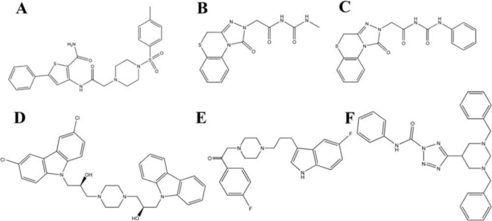
With respect to the obtained results, compound 38472 (maybridge code) was selected for further evaluation. As reported in
Table 7, some compounds have more negative estimated binding affinity value than -7.5 which their 2D structures are reported in
Figure 4.
Lead molecules retrieved from the database searching as potent glucagon receptor antagonist. (A) Compound C38472 (B) compound C26319 (C) compound C26315 (D) compound C 19450 (E) compound C 39388 and, (F) compound C 24155
On the basis of binding affinity, the order of compounds is: C38472> C26319> C26315> C19450> C39388> C24155
As it is obvious, compound C
38472 interacts more strongly with glucagon receptor site than the other compounds. The binding modes and molecular interactions between compound C
38472 (
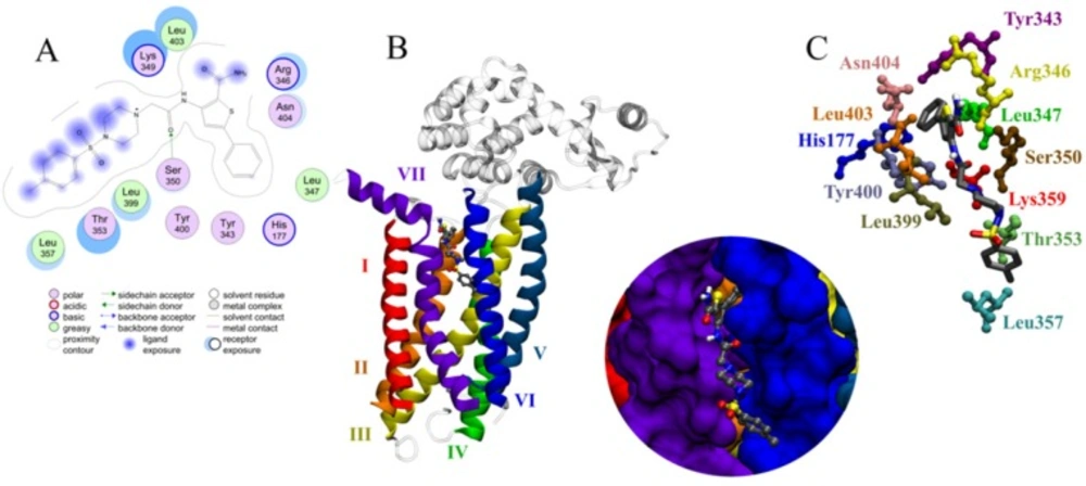
Figure 5) (with more binding affinity) and the active site components are discussed below.
As reported in literature (
62) the X-ray diffraction studies showed that the residues in outside of the seven transmembrane (7TM) helical bundle in a position between TM6 and TM7, extending into the lipid bilayer, play an important role in the ligand binding.
Molecular docking results (A) 2D representation and (B, C) 3D representation of docked orientations of C38472 in the binding site of glucagon receptor
Compound C
38472 has a free energy of binding of -7.9 kcal.mol
-1 and was in contact with the important residues of glucagon receptor such as Ser350, Leu399, Asn404, Thr353 and Lys349 (shown in
Figure 5).
Results of docking study showed that interactions were dominated by the hydrophobicity and aromaticity due to the presence of phenyls, amines, carbonyl and thiophenyl moieties.
The phenyl and thiophenyl rings of compound C38472 is situated in the pocket with high degree of hydrophobic property. This pocket includes the side chains of residues Leu 347, Ser 350, Tyr 400 and Tyr 343.
The carbonyl group between piperazine and amine group of C38472 has shown a hydrogen bond interaction with the backbone of SER350.
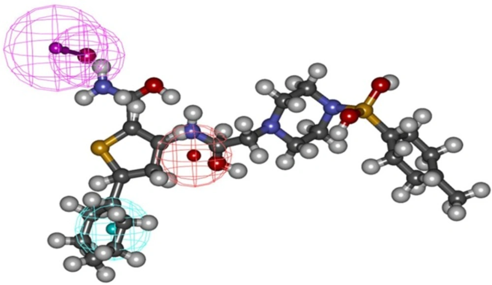
Binding mode of the compound C
38472 correlated well with the pharmacophore overlay (
Figure 1).
These findings well corroborates with the best pharmacophore hypothesis where the importance of hydrophobic functionality at the active site has been described by HYDROPHOBIC feature while H-bond interactions at the binding site has been well described by two HBD feature of the pharmacophore (
Figure 6).
The pharmacophore overlay of the compound C38472 on the Hypo1