3.1. Ex-Vivo Study
This study was approved by the ethical committee of the All India Institute of Medical Sciences (AIIMS), New delhi, India. Left coronary artery of 59 subjects were dissected while the cadavers were fresh (the time elapsed from the time of death was under 24 hours). The excised coronary arteries were from 6 females and 53 males with the age ranges between 20 and 70 years. Samples were selected from the left part of the heart containing left coronary ostium, left main coronary artery (LMCA), left anterior descending artery (LAD), and part of the left circumflex (LCX) of the human cadaver. This selection was based on the prevalence of the plaque on the left coronary artery especially in its proximal segment. Coronary artery samples were extracted from the cadavers who had died from a non-cardiac event. Samples were kept in 0.9% normal saline and refrigerated at 4 degrees Celsius. Maximum duration from the extraction of sample from cadaver and scanning time was 4 hours.
Coronary artery samples were removed from saline just prior to scanning. Left coronary artery was washed by injection of normal saline into the left coronary ostium in order to remove the blood from the coronary arterial lumen. Viscous solution of contrast agent (300 mgI / ml Ominpaque) was prepared by mixing methyl-cellulose with the solution iodinated contrast material in distilled water. The concentration of the viscous material was 2% weight by weight. The CT slices produced by this concentration were accepted by the cardiac radiologist for coronary artery wall evaluation (
Figure 1A-C). The viscous form of the contrast could be easily injected into the coronary artery by inserting the tip of the syringe into the left coronary ostium. Injection was stopped when the leakage of contrast material was seen from the end of the coronary artery branches. Small amounts of contrast, ejected due to leakage were removed very carefully from the end of the coronary artery branches.
Contrast material in a viscous form was retained in the coronary artery during the scanning procedure. Also, it coats the coronary artery wall permitting better visualization of the coronary artery wall.
Each sample was placed on the scanning table to mimic the process of scanning a real patient for coronary CT angiography (CTA). The coronary ostium was placed in the cranial position and the length of the LAD was oriented along the z-axis of the scanner.
Ex-vivo samples were scanned by Dual Source CT SOMATOM Definition Syngo CT 2008G (Siemens AG, Wittelsbacherplazz, DE-80333 Munchen, Germany). PBV protocol was used to scan coronary artery sample. This protocol uses 100 and 140 kVp, 64 × 0.6 mm beam width, pitch of 0.25, 0.33s rotation time, automatic tube current modulation (typical mAs values were 15), and the data collected at 360 degree was used to reconstruct the CT images. This protocol uses a demo electrocardiogram (ECG) with 60 beats/minute. B26f convolution kernel was used to reconstruct CT images with 0.6 mm slice thickness. Data collection diameter or scan field of views (SFOV) were 50 cm in all cases. Matrix size was 512 × 512 and MMWP workstation was used to perform DECT post processing on the raw data.
Two cardiac radiologists with more than 3 years of experience were asked to interpret the images independent of each other and they were blinded to the final pathology result.
On our suggestion to select only non-calcified plaques, the cardiac radiologists rejected the ex-vivo CT images when they could identify any trace of calcification in coronary artery plaque images.
Maximum intensity projection (MIP) and multi-planar reconstruction (MPR) were used to evaluate the presence of the non-calcified plaque throughout the coronary artery lumen by the cardiac radiologist. Actually, all cases where non-calcified plaque were found in the proximal part of LAD and bifurcation of LMCA and LCX, non-calcified plaques were seen identically in MIP images and MPR views. Therefore, MIP images were used to determine the position of non-calcified plaque for future visual assessment (
Figure 1B) in the present study. It has to be mentioned that MIP views were used only to assess the presence of non-calcified plaque. Therefore, we were not interested in any data such as slice thickness of the MIP images as they were unnecessary for the inversion procedure. Also, we reminded ourselves again that we were searching the non-calcified plaque in the proximal segment of the LAD and in the region of LMCA and LCX bifurcation portion. Visual evaluation was used in this study to verify the adequacy of DECT images to detect non-calcified plaque. Cardiac radiologist used true axial images (
Figure 1C) that were made on the basis of MIP images to evaluate and characterize the type of non-calcified plaque.
Gross photograph (A), maximum intensity projection (MIP) CT image (B) and axial CT image (C) of non-calcified plaque (shown by arrow adjacent to contrast agent inside the lumen). This sample was collected from a 58-year-old man. Based on the histopathology report, this is a fibro-lipid with a thin fibrous cap, and spotty calcification.
True axial images from the whole length of the non-calcified plaque were used to measure the density or HU value of the non-calcified plaque at two different energies (100 and 140 kVp) in each slice. Size of the region of interest (ROI) is a very important factor in our study. The size of the ROI was selected on the basis of the size of the non-calcified plaques. ROI had to be inside the plaque and should not contaminate the neighbouring structures, avoiding partial volume effect. The typical size of the selected ROI was between 1.1 and 5mm2. CT images that did not allow more than 3 pixels in the ROI were excluded from this study. The mean and standard deviations of the HU values for the circular ROI were measured three times for each slice to enhance its reliability. Each ROI contained minimum 3 pixels to prevent statistical uncertainty.
HU values of the structures surrounding the non-calcified plaque such as the border of the wall of the coronary artery, the fat surrounding the coronary artery wall, and the contrast material inside the lumen of the coronary artery were measured at 100 and 140 kVp to evaluate the possibilities of the overlapping (cross-reading) between the HU values of these structures in DECT images (
Figure 2).
Samples of the coronary artery which were categorized to have non-calcified plaque (by the cardiac radiologist) were cut cross-sectionally and thin tissue sections were obtained from the center part of the plaque (
Figure 1A). These samples were preserved in 10% formalin and sent to the pathology department. Samples were fixed in paraffin, cut into 5µm slices and stained by hematoxyline eosin for histologic evaluation of the plaque.
The location of the region of interest (ROI) which are used to measure the Hounsfield unit (HU) value on the fat surrounding coronary artery, the border of fat and wall of the non-calcified plaque, and contrast material in the lumen of coronary artery close to plaque.
3.2. Experimental Study for DECT Calibration
In this study, chemical compounds with known effective atomic number (Z
eff) and electron density (
ρe) were used to calibrate the DECT machine. These calibration samples were prepared by using high-purity samples of water, methanol, and acetic acid. Apart from these pure compounds, we also prepared aqueous solutions of glucose, sucrose, glycerol, citric acid, hydrochloric acid, and potassium hydroxide (
19) in suitable compositions. These chemical compounds were selected due to similarity of their Z
eff and
ρe values with those of the typical substances that are present in non-calcified plaque. Chemicals were of analytical purity and were purchased from Merck Chemicals Company. The details of the experimental work are described in Ref. (
20). These chemical solutions of known composition were filled in test tubes which were placed at the center of a water filled phantom, the test tubes being thus immersed in water. Both the phantom and test tubes were made of Poly Methyl Methacrylate (PMMA).
Different concentrations of known chemical solutions were prepared (in weight/weight %) by using digital balance (DENVER Instrument MXX 123, Gottingen, Germany) with 0.01 mg accuracy. Temperature measurements during the experiments were done by using a digital thermometer (Nuclear Associates 07 - 402, Hicksville, NY) with ± 0.5°C accuracy. Temperature of the CT room during experiments was fixed at 22 ± 0.5°C. The standard method, based on the use of specific gravity bottle, was employed to measure the density of all chemical solutions. The error in density measurement was less than 1%.
Test tubes were filled with liquid samples in pure form and as aqueous mixtures and inserted into the water filled phantom. The phantom containing test tubes was next placed on top of the scanning table in such a way that the length of the test tube was aligned along the Z axis of the scanning table and was perpendicular to the scanning plane
Figure 2 in Ref (
20). The phantom and all the samples in the test tubes were scanned by Dual-Source CT which would also be used subsequently to scan the ex-vivo coronary artery samples. For calibration, the phantom was scanned at 100 and 140 kVp and axial slices of the chemical compounds were reconstructed by 5 mm slice thickness. The circular ROI was placed at the center of each test tube, inside the chemical solutions, without contamination with the neighbouring structures. Mean and standard deviation of HU values were recorded for each ROI. The same procedure was repeated three times and average HU values from these three observations were used to enhance the validity of statistical estimations and analysis. For the same reason, care was taken to select a circular ROI containing 104 pixels in all measurements; thus, statistical fluctuations being minimal. The maximum standard deviation for the selected ROIs was 12. This shows that the maximum error on the mean value of the HU was 0.32%. Thus, from Equation 21 (
20) we calculated the error in the mean HU value to be typically 0.32%- which is acceptable.
3.3. Theoretical Background for DECT Inversion
The HU(V1) and HU(V2) (V1 = 100 and V2 = 140kVp) values of the known chemical compounds (ρe, Zeff) were used to calculate the DECT inversion coefficients. As is known, the HU(V) of the scanned sample is expressed by Equation (1):
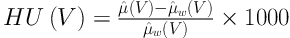
Where µ̂(V) and µ̂w(V) are the average linear attenuation coefficients of scanned material and water, respectively. It is known that the linear attenuation coefficient of the scanned material is a function of energy of the x-ray photons, effective atomic number and electron density of the scanned material. Linear attenuation coefficient in the range of x-ray energies used in diagnostic radiology (such as CT scanning) is given by Equation (2):

The linear attenuation coefficient due to Compton scattering is weakly dependent on the
energy of the x-ray photons, and directly proportional to the electron density of the material.
Photoelectric absorption, on the other hand, depends strongly on the x-ray photon energy (E) and the effective atomic number of the material, the dependence being (ρe × (ZeffX) / E3). Since the x-ray photons produced by x-ray sources are not monoenergetic, the HU(V) given by the CT machine describes the attenuation coefficient, µ̂(V), averaged over the source spectrum.
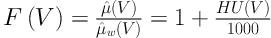
From Equation 1, we can define a quantity F(V) to be in Equations (3) and (4)
and

where the first term is the contribution from Compton scattering and the second term is from the photoelectric effect. Thus, by taking the ratio of F(V1) and F(V2) for two different excitation voltages of the x-ray tube we get,
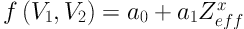
which depends on Zeffx alone, ρe being eliminated, where we have defined f (V1, V2) by Equation 6:
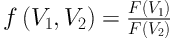
Thus, if the coefficients a0 and a1 are known, we are able to determine (Zeffx) of the substance, from the experimental values of f (V1, V2), where f (V1, V2) is calculated from the observed HU(V1) and HU(V2) values of the substance.
For finding the inversion coefficients, a0 and a1, we take samples with known values of (Zeffx) and measure their HU(V1) and HU(V2) with the CT machine that is being calibrated. From these HU values, f (V1, V2) are calculated and fitted to Equation 5. With a0, a1 determined, Equation 4 serves as the inversion algorithm for (Zffx).
From our numerical study of the photoelectric mass attenuation coefficients of substances with different Zeff values, we found that Zeff is related to (Zeffx), as is shown by Equation 7:
where the values of the mass attenuation coefficients were taken from the NIST tables.
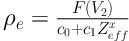
The value of Zeff being known, we have to address next the task of finding the electron density, ρe. On defining, Y = F(V2) / ρe and X = Zeffx we find that we can write Equation 8:
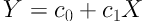
By making least square fit of the data with Equation 8 for known chemical compounds, the coefficients c0 and c1 can be calculated. This method becomes accurate when HU values of the higher kVp (for example 140kVp) are used, since at those energies photoelectric effect is insignificant and Zeffx has hardly any contribution to the HU values. Once c0 and c1 are determined from the data, Equation 8 is the inversion algorithm for finding (ρe). In other words,
HU(V2) of unknown materials can be used in Equation 8 to predict ρe to be,


, maximum intensity projection (MIP) CT image (B) and axial CT image (C) of non-calcified plaque (shown by arrow adjacent to contrast agent inside the lumen). This sample was collected from a 58-year-old man. Based on the histopathology report, this is a fibro-lipid with a thin fibrous cap, and spotty calcification.")
 which are used to measure the Hounsfield unit (HU) value on the fat surrounding coronary artery, the border of fat and wall of the non-calcified plaque, and contrast material in the lumen of coronary artery close to plaque.")
 and HU(140) for each slice in true axial CT images measured through the whole length of non-calcified plaque (A) and neighbouring structures of the non-calcified plaque such as fat surrounding the coronary artery (B), border of fat and wall of the coronary artery, non-calcified plaque and contrast material inside the lumen of the coronary artery (<a href=\"#A13970REF19\">19</a>)")
 versus HU (140) of the chemical compound used for calibration inversion purposes (<a href=\"#A13970REF19\">19</a>)")
 versus HU (140) of 208 data points of non-calcified coronary artery plaques belonging to 21 human heart cadaver samples")
; and Region D: there is no sample")
