1. Background
Chest X-ray (CXR), an imaging test, assesses the tissues and structures in the chest using X-rays. It helps medical professionals detect abnormalities in the heart and lungs. The lungs may change as a result of certain heart issues, and specific disorders may cause anatomical alterations of the heart or lungs. In standard clinical practice, a CXR or chest radiography is the initial diagnostic tool applied for patients demonstrating non-specific thoracic symptoms (e.g., chest pain, cough, or shortness of breath). Most institutions can easily perform chest radiography at a low cost and with efficiency. Several studies have been conducted in this area, and radiologists face a practical issue in maintaining diagnostic quality due to the volume of chest radiographs that require interpretation. Lesions that were initially missed are often detected retrospectively, even when an experienced radiologist performs the initial assessment.
Kang et al. (1) introduced a state-of-the-art encoder-decoder-based network with an attentional decoder explicitly designed to accurately detect small lesions in images. Traditional networks with encoder-only architectures frequently struggle with minor lesions, as these can become vague during down-sampling or within low-resolution feature maps. The proposed network addressed this issue using an encoder-decoder architecture comparable to the U-Net family, enabling it to process images and classify lesions by globally pooling high-resolution feature maps. Further, two main challenges arose in adapting U-Net designs for classification tasks in the same survey study (2). The first challenge is the high computational costs for up-sampling, and the second is finding a computationally light pooling method that could improve object localization. Deep residual learning can be applied to shallow layers with high-resolution feature maps to tackle these problems. Their proposed network includes a harmonic magnitude transform and a lightweight attentional decoder. By decoupling low-resolution features from those at high resolution to be used as keys and values, the attentional decoder up-samples the characteristics. This multiscale interaction enables the upsampled features to retain the characteristics of local lesions, thereby helping to maintain the global context. Furthermore, the spatial frequency representation is used to extract high-resolution feature maps through pooling via the harmonic magnitude transform (3-5). This method reduces the parameters required for the pooling layer with an efficient embedding scheme and simultaneously retains the shift-invariance using the shift theorem of the Fourier transform. The results of the experiments on the three publicly available CXR datasets, NIH (6), CheXpert (7), and MIMIC-CXR (8), show that this network ranks at the state-of-the-art level in terms of lesion classification. Hence, the encoder-decoder network proposed in this paper provides great support for solving the problem of automatically classifying X-ray images with small lesions by achieving performance improvements with both feature maps at multiple resolutions upsampled back to the input resolution through an attentive decoder and high-resolution feature maps processed via the harmonic magnitude transform.
Innat et al. (9) demonstrated Cardio-XAttentionNet, a deep learning network that accurately categorizes and detects the presence of cardiomegaly in CXR images using convolutional attention mapping. The model aims to help doctors and improve patient care through knowledgeable disease categorization. Furthermore, it assists in locating the illness. A weighting term was appended to the conventional global average pooling (GAP) system (10), whereas this simple attention mapping mechanism was optimal. This innovation enables Cardio-XAttentionNet to locally classify images at the image level and locate cardiomegaly regionally at the pixel level without requiring challenging pixel-level annotations.
Cardio-XAttentionNet was trained with the ChestX-ray14 dataset, a publicly accessible collection of CXR images, and is based on sophisticated convolutional neural network (CNN) architectures. The model’s performance metrics were remarkable. Cardiomegaly classification achieved precision, recall, F1 score, and area under the curve (AUC) scores of 0.87, 0.85, 0.86, and 0.89, respectively. The results indicate that Cardio-XAttentionNet accurately determines the condition at the pixel level in addition to classifying cardiomegaly at the image level. Cardio-XAttentionNet exhibits state-of-the-art performance in cardiomegaly diagnosis when compared to current GAP-based models, highlighting its potential as an effective tool in medical diagnostics.
Wang et al. (11) accentuated the serious effects of the coronavirus disease 2019 (COVID-19) pandemic on world health and stressed the importance of operational screening techniques, especially those that use chest radiography. Early examination revealed that CXR images of patients with COVID-19 display specific anomalies. An extensive open-access benchmark dataset of 13,975 CXR images from 13,870 patient cases is introduced in the review. At the time of its release, this dataset contained the largest number of publicly available cases that tested positive for COVID-19. The scientists used a logical strategy to determine the fundamental attributes associated with COVID-19 cases, allowing them to further explore how coronavirus net generates its predictions. This strategy ensures that coronavirus net’s selections are based on significant CXR image data and assists clinicians in improving their screening techniques. Indeed, although coronavirus net is not yet ready for production use, its open-access design and the COVIDx dataset make it a significant tool for resident data scientists and corresponding researchers. This aims to facilitate the advancement of highly accurate and useful learning techniques for COVID-19 case detection, which will eventually enable people in dire need to receive treatment quickly.
Nair et al. (12) revealed that the availability of portable devices and the popularity of chest radiology systems in healthcare facilities allow radiography exams to be performed rapidly and broadly. This makes them a great addition to reverse transcription polymerase chain reaction testing, especially since CXRs are a frequent routine procedure for patients with respiratory problems. Subsequently, de Hoop et al. (13) focused on the commercially available CAD system, Onguard 5.0 by Riverain in Miamisburg, Ohio, and revealed no significant improvement in viewers’ ability to determine malignancy in chest radiographs. This best illustrated the limitations of the system in the absence of deep learning, as observers found it challenging to discern true lesions from false positives. A wide series of consecutive chest radiographs indicated that a stand-alone CAD system had a sensitivity of 71.0%, with 1.3 false positives per image, according to a recent study by Li et al. (14). However, the more recent nodule detection computer-aided diagnosis system, ClearRead +Detect 5.2 (previously Onguard from Riverain Technologies), performs better despite the absence of deep learning. Its wide adaptation in clinical settings still requires higher sensitivity and fewer false positives.
2. Objectives
The objective of this study is to enhance the classification accuracy of CXR images, particularly for identifying eight types of abnormal lung lesions, by applying advanced feature selection and fusion techniques in combination with deep learning models. Our study significantly contributes to the realm of medical image analysis by introducing a detailed methodology for the accurate classification of CXR images by harnessing the capabilities of two sophisticated deep learning architectures, ResNet50 and DenseNet201. Furthermore, using transfer learning (TL), we develop robust feature representations of CXR images.
The proposed work introduces a novel and efficient framework for classification, which is as follows:
- Initially, in our workflow, the crucial step is the preprocessing of data, which is meticulously designed to refine and improve the raw data, ensuring it is clean, consistent/reliable, and properly organized for optimal performance when fed into the deep learning models.
- For the extraction of features, we used two deep learning models (ResNet50 and DenseNet201) and then trained them using TL separately.
- We utilized the output and fetched separately under two feature vectors and applied the parameter-optimized ant colony optimization (ACO) algorithm for optimal feature selection.
- In the meantime, five additional statistical methods, which include the Kruskal-Wallis test, ReliefF, analysis of variance (ANOVA), chi-square test, and minimum redundancy maximum relevance (MRMR) for the most important features, are used at the preprocessing step, separate from the above process.
The fusion process is enforced after obtaining important features from two different processes to improve the efficiency of our architecture. The optimized deep features (ACO) and the statistically selected handcrafted features were fused at the feature level via horizontal concatenation, producing a comprehensive hybrid vector. We then used various machine learning classifiers.
3. Materials and Methods
3.1. Preprocessing
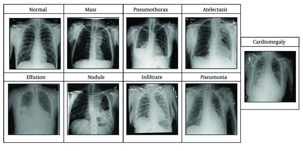
The dataset (15) includes eight lesions, namely cardiomegaly, effusion, infiltrate, mass, nodule, atelectasis, pneumonia, and pneumothorax, as illustrated in Figure 1.
Cardiomegaly can be identified by an enlarged cardiac silhouette on an X-ray. More clearly, it indicates that the heart appears larger than it usually is, may occupy more than half of the thoracic width, and enables more prominent heart border visualization. Pneumonia can be determined by the presence of dense lobar, segmental, or patchy opacities. Effusion can be identified by the presence of fluid in the pleural space; briefly, the fluid curves upward sideways on the lung edges. Infiltration is identified as increased opacity due to fluid, pus, blood, or cells within lung tissues. A nodule is a small, round opacity that is less than 3 cm in diameter, with sharp margins. A mass is larger than a nodule and has comparable properties; thus, an opacity greater than 3 cm is considered a mass. Pneumothorax is identified by the presence of air in the pleural space, causing the affected lung to appear darker and retracted from the chest wall, where the lung is collapsed. Atelectasis is determined by compensatory overinflation of the adjacent lung, and the affected area appears opaque.
We used the NIH ChestX-ray14 dataset, which comprises 112,120 frontal-view X-ray images from 30,805 unique patients, each image categorized with one or more of 14 thoracic disease categories such as atelectasis, cardiomegaly, effusion, infiltration, mass, nodule, pneumonia, pneumothorax, consolidation, edema, emphysema, fibrosis, pleural thickening, and hernia. The images are provided in JPEG format with a resolution of 1024 × 1024 pixels. In our case, we used only eight thoracic disease classes: Atelectasis, cardiomegaly, effusion, infiltration, mass, nodule, pneumonia, and pneumothorax. The total number of images used was 66,392, and the splitting ratio carried through our experiment was 70:10:20. We used 70% for training purposes, 10% for validation, and 20% for testing. For training purposes, we used 42,042 X-ray images, followed by 6,006 X-ray images for validation purposes, and lastly, for testing, we used 12,012 X-ray images. For binary classification, the data were grouped into normal images labeled as "No Finding" and abnormal images with one or more pathologies, resulting in 60,361 normal and 51,759 abnormal images.
3.2. Feature Fusion and Classification
In our study, we utilized a CXR dataset comprising normal and abnormal classes. We precisely preprocessed the images, and subsequently, deep learning models required fixed-size inputs. All images in the dataset were resized to a uniform dimension, ensuring consistency and allowing the model to learn representative features efficiently. The original images were of size 1024 × 1024 pixels, and after augmentation, the image dimensions were adjusted to 948 × 948 pixels to optimize the dataset for deep learning models. For model compatibility, all images were resized to 224 × 224 pixels. This step ensures consistent data distribution, which helps accelerate the training process and improves model efficiency.
Various augmentation techniques were applied, including cropping, which focused on critical regions of the images, ensuring only relevant areas are used for training. Random rotation was applied, with images randomly rotated between 30° to 60°, enhancing the model's ability to generalize across various orientations. Zoom transformation was applied randomly within a range of ± 20% to simulate varying scales, and lastly, horizontal and vertical flipping were performed randomly to diversify the dataset and increase robustness. The resolution of the images was maintained for both horizontal and vertical resolutions to preserve image clarity and feature details.
To improve generalizability and prevent overfitting, data augmentation techniques were applied to enhance model robustness by artificially increasing the diversity of the training set. Pixel intensity values were normalized to a range of 0 - 1 or standardized (zero mean, unit variance) based on the model’s requirement. ResNet and DenseNet require input images to be normalized to a range of 0 - 1 or standardized using mean subtraction and standard deviation (SD) division. This step ensures faster convergence during training and prevents numerical instability by keeping the values within a manageable range. Therefore, the preprocessing includes resizing, normalization, and augmentation to improve the model’s robustness and accuracy. Our approach involves preprocessing the data to ensure that it is optimal while feeding it to deep learning models using two deep learning architectures, ResNet50 and DenseNet201, tailored to our specific classification task. Through TL, we fine-tuned these pretrained models on our CXR dataset, extracting features that serve as rich representations of the images, capturing crucial patterns and characteristics.
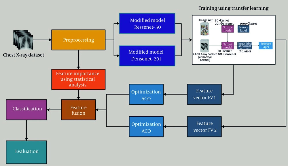
We used a two-step feature selection and fusion approach to improve classification performance and efficiency. In the initial step, we utilized two modified deep learning models to extract deep features from the CXR images. The extracted feature sets were stored separately as feature vectors [FV1 (ResNet50) and FV2 (DenseNet201)]. To refine the extracted features, we applied a parameter-optimized ACO algorithm to each feature set separately. We have not changed the core structure of ACO; instead, we used the term "parameter-optimized ACO" to denote the parameter optimization executed on the standard ACO algorithm. The mechanics of ACO were well-maintained, but numerous key control parameters, including the number of ants (N), heuristic factor (β), pheromone influence (α), pheromone evaporation rate (ρ), and the number of selected features (Nf), were carefully adjusted. The ACO helps in selecting the most relevant and discriminative features while reducing dimensionality, thereby ensuring that only essential features contribute to classification.
In parallel, we applied five statistical methods (Kruskal-Wallis test, ReliefF, ANOVA, chi-square test, and MRMR) to select the most significant features from the dataset. This statistical feature selection process was performed independently from the ACO to provide an additional level of refinement. After obtaining the crucial features from both ACO-selected deep features and statistically selected features, we performed feature fusion by combining these refined feature vectors into a single feature set. This fusion technique ensures that the final feature set retains both deep learning-based high-level patterns and statistically significant handcrafted features. The fused feature set was then used as input to various machine learning classifiers, which improves both the classification accuracy and efficiency. Figure 2 illustrates the proposed flow diagram of our CXR classification using a hybrid approach.
The CNNs, which perform well in tasks such as image recognition (16, 17), image classification (18), and object detection (19), are among the most important types of deep neural networks. Compared to other classification techniques, CNNs require less preprocessing. This network categorizes an image into distinct classes based on its input. Convolutional, pooling, ReLU, fully-connected, and softmax layers are among the many layers that the images travel through in both the training and testing stages. Using convolutional filters, image pixels are transformed into features in the convolutional layer, whereas the softmax layer assigns probabilities to these features, ranging from 0 to 1, for classification.
ResNet exhibits superior performance due to its ability to establish a more direct information propagation path across the network. Its design effectively mitigates the vanishing gradient issue encountered in backpropagation. By introducing shortcut connections, ResNet facilitates the passage of relevant information throughout the training process, thereby circumventing unhelpful layer interactions. Mathematically:
Equation 1.
Equation 2.
Both Equations signify signify the residual mapping mechanism in ResNet. The primary idea behind ResNet is to reformulate learning as learning residual functions, which helps preserve relevant information across layers. Specifically, Equation (1) describes how a transformation function T(i) can be modeled as a residual function R(i), where the identity mapping i is subtracted. In Equation (2), it expresses the inverse relation, thereby reinforcing how residual learning captures essential variations while maintaining identity connections. These Equations are are decisive in understanding how ResNet shortcut connections enable effective gradient flow and mitigate vanishing gradients.
We utilized 64 kernels with a 7 × 7 convolutional layer, a stride of 2, a 3 × 3 max pooling layer, a 7 × 7 average pooling layer with a stride of 7, 16 residual building blocks, and a fully connected (FC) layer in our research using the ResNet-50 pretrained model. This network design exhibits extraordinary versatility with over 23 million trainable parameters. The model was then adapted by eliminating its final FC layer. Initially, this layer encompassed 1000 object classes. However, to align with our selected CXR dataset, consisting of only two classes, we introduced a new FC layer accommodating only two classes. This modified configuration underwent training using deep TL techniques, as elaborated in the subsequent section. After the TL process, we derived a refined model. Subsequently, from the GAP layer, this refined model was employed to extract features, and N times 2048 is the dimensionality of the extracted features. Figure 3 illustrates the CNN architecture for the CXR dataset.
This network involves 201 deep layers. It was initially trained on a thousand object classes, and the ResNet model introduced the idea of bypassing layers, in contrast to other deep networks where layers are connected progressively, making the system more complex and difficult to use. Subsequently, the DenseNet network improved upon this strategy by using sequential concatenation in place of the output feature summation from previous layers (20). Further, mathematically, it can be defined as follows.
Equation 3.
In this Equation, the the features of the ɭth layer are represented by Zɭ, the Layer Index is denoted by ɭ, and Hɭ is a nonlinear transformation. Dense blocks are established in the architecture for down-sampling. These blocks are then isolated by layers called transition layers, which include batch normalization. A 1 × 1 convolution layer and a 2 × 2 average pooling layer follow the transition layers. The DenseNet-201 architecture uses pooling blocks, which are designed to reduce the size of the feature maps. Each layer within DenseNet has direct access to the original input image and the gradients from the loss function, resulting in a notable reduction in computational speed.
DenseNet201 was modified for CXR classification in this study. The FC layer, initially designed for 1000 object classes, was eliminated and replaced with a novel FC layer accommodating only two classes. The modified model then underwent training using TL. During training, the model ran for 100 epochs, with a learning rate set at 0.00001. We employed stochastic gradient descent for optimization, and the batch size was set to 64. After training, the newly distinguished model was saved for subsequent feature extraction. Finally, features were extracted from the GAP layer, which was then used for chest abnormality classification purposes.
3.3. Deep Feature Extraction
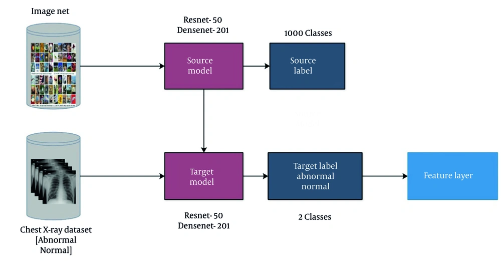
The TL in the domain of deep learning involves repurposing a model for a specific task (21). TL primarily aims to exploit a preexisting model instead of constructing a new one from scratch. Throughout this process, base models, alongside their corresponding labels and data, are considered. Subsequently, the knowledge is transferred to the adapted model, which is trained for the new task. The training process required certain parameters, including 100 epochs, a learning rate of 0.00001, and stochastic gradient descent, with the batch size set to 64. The modified models that have undergone training were saved for deployment in the intended task.
TL encompasses leveraging the knowledge gained from pretrained models on a source task and applying it to a related target task. Mathematically, TL can be represented as follows.
Equation 4.
In this Equation, let let fs represent the pretrained model on the source task, and let ft represent the target task model. Feature extraction involves extracting informative features from the input data, which can then be utilized for classification or other tasks.
Figure 4 illustrates the TL process. Furthermore, the source models in this figure have a total of 1000 object classes. Knowledge is transferred, and modified models are trained in TL. After the training of both models, the features are extracted from the final layers (global average pool) and applied to the subsequent step. The retrieved feature vectors from each layer have sizes of N times 2048.
3.4. Statistical Feature Selection
In this section, we discuss the mathematical representation of some of the statistical methods used to rank the importance of features. The methods include the Kruskal-Wallis test, ReliefF, ANOVA, chi-square test, and MRMR.
Kruskal-Wallis test: The Kruskal-Wallis test is the nonparametric version of ANOVA used to compare the distribution of features across classes, which will be referred to as normal and abnormal in our case. The test statistic can be calculated as follows.
Equation 5.
Where Ri is the sum of the ranks for the ith group (which are normal and abnormal), ni is the number of observations in the ith group, and N is the total number of observations.
Degree of freedom: Mathematically, it can be defined as follows.
Equation 6.
Where k is the number of groups (there are two in our case: Normal and abnormal). A higher value would indicate a greater difference between normal and abnormal classes.
ReliefF: This is an instance-based method that primarily aims to assign weights to features based on their ability to distinguish between normal and abnormal instances. For each instance Xi, finding the nearest hit means the same class, and the nearest miss indicates a different class. Afterward, the weight for feature X is updated. Mathematically, it can be defined as follows.
Equation 7.
Where Δ(X, hit) and Δ(X, miss) are the differences between the feature values of X and its nearest hit and miss, respectively. Higher weights denote more important features for distinguishing between normal and abnormal classes.
The ANOVA: This method is used to determine any statistically significant variances between the means of the normal and abnormal classes. The main mathematical equation for this method is defined as the F-statistic as follows.
Equation 8.
Where mathematically, mean square between groups (MSB) is defined as follows.
Equation 9.
For mean square within groups (MSW), it can be defined as follows.
Equation 10.
Degree of freedom: Here, we can describe it by two Equations: One One would be considered as between the groups and the other would be within the groups. Mathematically, we express it as follows.
Equation 11.
Equation 12.
In Equation 11 and Equation 12, k is the number of classes, and in our case, it is 2 (normal and abnormal), and n can be described as the number of samples. Now we know the standard equation for SSB, which is defined as the sum of squares between the groups, and SSW, which is the sum of squares within the group. A clear mathematical representation is presented as follows.
Equation 13.
Now, as we have two classes, according to our requirements, the above SSB and SSW mathematical representation would be defined as in the below two Equations (15) and (16).
Equation 15.
Where n1 and n2 are the number of samples, and C1 and C2 are classes, respectively.
Equation 16.
Where
The five filter-based statistical feature selection methods used in our study — Kruskal-Wallis, ANOVA, chi-square, ReliefF, and MRMR — were implemented using MATLAB’s classificationLearner and fsc functions. Each method ranked features based on its respective scoring metric. The non-parametric one-way ANOVA, based on the H-statistic, used MATLAB's kruskalwallis ranking function to score each feature. For ANOVA, features were scored based on their F-statistic, reflecting between-group vs. within-group variance, and top features with the highest F-values were retained using MATLAB’s fscAnova function. For the chi-square test, we evaluated statistical independence between each feature and the class label using MATLAB’s fscchi2 to score features. ReliefF, a nearest-neighbor-based method, assigns weights based on a feature’s ability to distinguish between similar instances from different classes using relieff with default settings. For MRMR, which balances relevance (via mutual information with class labels) and redundancy (via correlation with other features), we used MATLAB’s fscmrmr to rank the features and select the top features per method. These subsets were later merged via union, combining all unique features to form the handcrafted statistical feature set used in fusion.
The selection of these five methods was due to their diverse selection criteria and wide usage in biomedical research. The ANOVA and chi-square offer simple, univariate tests that are statistically robust for large feature sets, whereas Kruskal-Wallis adds a non-parametric alternative to ANOVA, helpful when normality expectations are not satisfied. ReliefF brings a local, instance-based perspective, which captures interactions better than purely statistical tests, and MRMR ensures a balance between relevance and low redundancy, important for avoiding correlated features. Their grouping provides a comprehensive selection framework that leverages both global and local relevance of features, ensuring robustness across feature types in medical datasets.
4. Results
This study aimed to investigate the performance of different feature selection methods and classifiers on a CXR radiography dataset containing normal and abnormal classes. The X-ray dataset was managed, and features were extracted using the pretrained deep learning models, DenseNet-201 and ResNet-50. Five statistical feature selection techniques were then applied to the extracted features. These five feature selection techniques are ANOVA, chi-square test, MRMR, ReliefF, and Kruskal-Wallis, used to determine the most informative features for distinguishing between the normal and abnormal X-ray images.
After feature selection, the most appropriate features were utilized to train and assess the performance of five classifiers: Linear support vector machine (LSVM), quadratic support vector machine (QSVM), cubic support vector machine (CSVM), medium Gaussian support vector machine (MGSVM), and ensemble subspace discriminant (ESD) model. The dataset was then divided into training, validation, and test sets with a 70:10:20 ratio to ensure robust model assessment. The classifiers were trained on the training set, and hyperparameter tuning was conducted using the validation set. The final performance assessment was conducted on the test set, focusing on metrics of the classifiers, such as accuracy, sensitivity rate, specificity rate, misclassification rate, F1 score, precision rate, and area under the receiver operating characteristic curve (AUC-ROC), individually.
The test outcomes were carefully examined to identify the best feature selection strategies and classifier combinations for detecting CXR abnormalities. The results demonstrate how various methods of machine learning may assist radiologists with diagnostic duties, as long as important new information regarding the use of machine learning in medical image analysis is gained. To ensure viable reproduction, the experiments were conducted with MATLAB2020a on a PC equipped with an Intel i7 CPU, 32 GB RAM, and an NVIDIA GeForce GTX 750 TI graphics card. Furthermore, the Matconvnet deep learning toolbox was used to perform deep feature extraction, which enhanced the system’s ability to recognize subtle patterns and attributes within the CXR data.
To determine the functional level of machine learning models in solving certain problems, their performance needs to be measured. We use certain predominantly utilized machine learning parameter metrics to assess our CXR classification system’s performance in a broad sense. These measures, along with the model’s accuracy in classifying cases of chest anomalies, provide insightful information about numerous facets of the model’s performance. Here, we discuss the parameter metrics that were used to compute performance: The AUC-ROC, F1 score, sensitivity rate, precision rate, specificity rate, and misclassification rate.
Sensitivity, also known as recall or true positive rate, assesses how well the model correctly identifies positive instances among all actual positive instances, calculated using Equation (17). Specificity, also known as the true negative rate, evaluates how well the model correctly recognizes negative instances among all actual negative instances. It is calculated using Equation (18). The misclassification rate, also identified as the error rate, measures the proportion of all instances (both positive and negative) that are incorrectly classified by the model. It is calculated using Equation (19). Precision, often denoted as a positive predictive value, estimates the proportion of accurate positive predictions out of all positive predictions made by the model, as calculated using Equation (21). The F1 score, a combination of precision and recall, provides a balanced measure of the model’s overall performance, accounting for both false positives and false negatives. It is calculated using Equation (22). The AUC-ROC measures the model’s ability to distinguish between positive and negative classes across various threshold settings. A higher AUC value signifies better discrimination capability, with 1 indicating perfect classification.
Equation 17.
Equation 18.
Equation 19.
Or simply by the equation:
Equation 20.
Equation 21.
Equation 22.
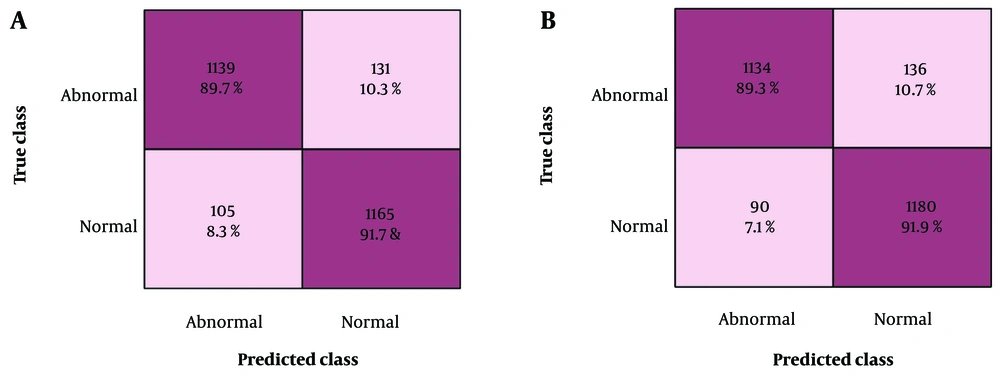
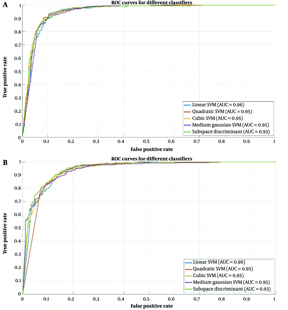
This study investigated the performance of different feature selection methods and classifiers on a CXR radiography dataset. Performance evaluation was conducted on the test set, focusing on metrics such as accuracy, sensitivity rate, specificity rate, misclassification rate, F1 score, precision rate, and AUC-ROC of the classifiers. The outcomes were carefully analyzed to identify the best feature selection strategies and classifier combinations for determining abnormalities in CXRs. Table 1 shows various machine learning classifiers, including LSVM, QSVM, CSVM, MGSVM, and ESD models, which were used to classify abnormalities in CXRs. LSVM achieved the highest accuracy of 90.7% and 91.1% on ResNet-50 and DenseNet-201, respectively.
| Variables; Classifier | Sensitivity rate (%) | Precision rate (%) | Specificity rate (%) | F1 score (%) | AUC | Misclassification rate (%) | Accuracy (%) | Time (s) |
|---|---|---|---|---|---|---|---|---|
| M-ResNet50-IACO (M-R50-IACO) | ||||||||
| LSVM | 91.64 | 89.73 | 89.97 | 90.67 | 0.96 | 9.291 | 90.7 | 30.599 |
| QSVM | 92.33 | 88.11 | 87.98 | 90.17 | 0.95 | 9.61 | 90.4 | 32.112 |
| CSVM | 91.71 | 88.81 | 89.16 | 90.24 | 0.95 | 9.601 | 90.4 | 36.864 |
| MGSVM | 91.65 | 88.11 | 88.55 | 89.85 | 0.95 | 9.960 | 90.0 | 38.216 |
| ESD | 90.59 | 87.95 | 88.29 | 89.25 | 0.93 | 10.59 | 89.4 | 192.68 |
| M-DenseNet201-IACO (M-D201-IACO) | ||||||||
| LSVM | 92.65 | 89.29 | 89.67 | 90.89 | 0.96 | 8.893 | 91.1 | 107.09 |
| QSVM | 92.64 | 89.13 | 89.53 | 90.85 | 0.95 | 8.980 | 91.0 | 22.671 |
| CSVM | 92.19 | 89.21 | 89.55 | 90.78 | 0.95 | 9.171 | 90.8 | 24.536 |
| MGSVM | 92.42 | 88.35 | 88.83 | 91.35 | 0.95 | 9.455 | 90.6 | 25.401 |
| ESD | 93.05 | 88.58 | 89.11 | 90.76 | 0.95 | 9.015 | 91.0 | 20.489 |
Abbreviations: AUC, area under the curve; IACO, improved ant colony optimization; M-ResNet50, modified ResNet-50; LSVM, linear support vector machine; QSVM, quadratic support vector machine; CSVM, cubic support vector machine; MGSVM, medium Gaussian support vector machine; ESD, ensemble subspace discriminant; M-DenseNet201, modified DenseNet-201.
Figure 5 presents the confusion matrix corresponding to the highest accuracy achieved, providing further insight into the model’s performance. The confusion matrix offers a detailed breakdown of the classifier’s predictions compared with the actual classes, thereby enabling a comprehensive assessment of the classifier’s classification accuracy. Figure 6 presents a graph comparing the AUC values that illustrate the performance of the five classifiers applied to features derived from the ResNet-50 and DenseNet-201 deep learning models.
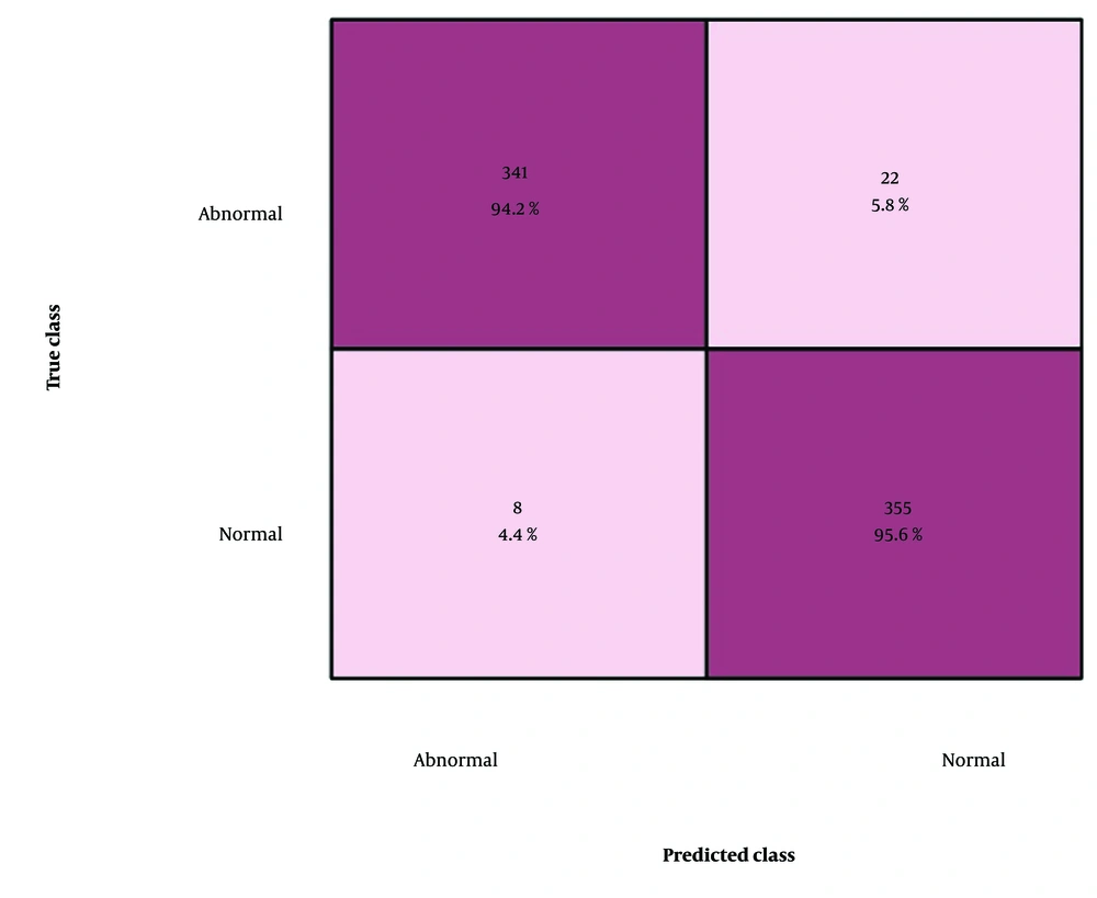
Table 2 shows that the fusion of both models and the ESD model achieved the highest accuracy of 95.9%, with a sensitivity of 97.70%, precision rate of 93.94%, specificity of 94.16%, F1 score of 95.78%, AUC-ROC of 0.99, and a misclassification rate of 4.13%, which was the lowest among all classifiers. Figure 7 illustrates the confusion matrix that provides a detailed breakdown of the classifier’s predictions compared with the actual classes, thereby enabling a comprehensive assessment of the classifier’s classification accuracy.
| Classifier | Sensitivity rate (%) | Precision rate (%) | Specificity rate (%) | F1 score (%) | AUC | Misclassification rate (%) | Accuracy (%) | Time (s) |
|---|---|---|---|---|---|---|---|---|
| LSVM | 95.76 | 93.39 | 93.54 | 94.56 | 0.99 | 5.43 | 94.6 | 31.825 |
| QSVM | 95.53 | 94.22 | 94.29 | 94.87 | 0.99 | 5.01 | 95.0 | 35.337 |
| CSVM | 96.03 | 93.39 | 93.57 | 94.69 | 0.99 | 4.79 | 95.3 | 24.291 |
| MGSVM | 94.72 | 93.94 | 93.99 | 94.33 | 0.98 | 5.60 | 94.4 | 26.924 |
| ESD | 97.70 | 93.94 | 94.16 | 95.78 | 0.99 | 4.13 | 95.9 | 16.511 |
Abbreviations: AUC, area under the curve; LSVM, linear support vector machine; QSVM, quadratic support vector machine; CSVM, cubic support vector machine; MGSVM, medium Gaussian support vector machine; ESD, ensemble subspace discriminant.
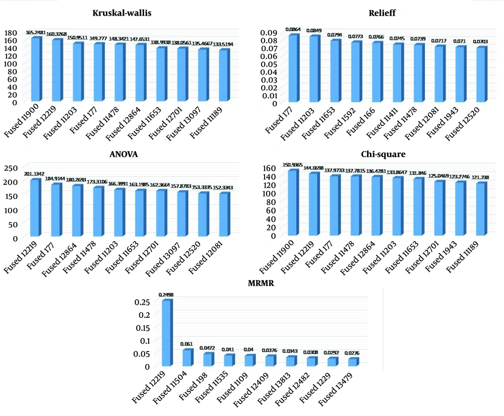
Table 3 shows the top 10 features using the above five methods, and these are after the fusion of two deep learning pretrained models, ResNet-50 and DenseNet-201, which were modified. The Kruskal-Wallis test, a nonparametric approach, assesses differences in feature distributions across classes, producing an H-statistic to identify feature relevance. ReliefF assesses features iteratively according to their capacity to differentiate between nearby instances of differing classes, assigning weights to features where higher weights indicate greater importance. The ANOVA examines variances between classes and identifies features that significantly contribute to class differentiation, calculating an F-statistic for each feature, with higher values indicating greater importance. The chi-square test evaluates the independence between features and the target variable, with higher chi-square values representing a stronger association with class labels and, thus, higher importance. The MRMR selects features that are highly relevant to the target variable while minimizing redundancy among features. This is achieved by balancing relevance and redundancy, maximizing mutual information with the target, and minimizing mutual information among selected features. We presented the top 10 features determined using the five feature selection methods, all of which were applied after the fusion of both models. Figure 8 illustrates the bar chart representations of the five methods.
| Features | Kruskal-Wallis | Features | ReliefF | Features | ANOVA | Features | Chi-square | Features | MRMR |
|---|---|---|---|---|---|---|---|---|---|
| Fused11900 | 165.2481 | Fused177 | 0.0864 | Fused12219 | 201.1342 | Fused11900 | 150.9365 | Fused12219 | 0.2498 |
| Fused12219 | 160.3268 | Fused11203 | 0.0849 | Fused177 | 184.9144 | Fused12219 | 144.0698 | Fused11504 | 0.0610 |
| Fused11203 | 150.9511 | Fused11653 | 0.0794 | Fused12864 | 180.2693 | Fused177 | 137.9733 | Fused198 | 0.0472 |
| Fused177 | 149.7770 | Fused1592 | 0.0773 | Fused11478 | 173.3106 | Fused11478 | 137.7815 | Fused11535 | 0.0410 |
| Fused11478 | 148.3421 | Fused166 | 0.0766 | Fused11203 | 166.3991 | Fused12864 | 136.4281 | Fused1109 | 0.0400 |
| Fused12864 | 147.6531 | Fused11411 | 0.0745 | Fused11653 | 163.1985 | Fused11203 | 133.8647 | Fused12409 | 0.0376 |
| Fused11653 | 138.9938 | Fused11478 | 0.0739 | Fused12701 | 162.3664 | Fused11653 | 131.8460 | Fused13813 | 0.0343 |
| Fused12701 | 138.0561 | Fused12081 | 0.0717 | Fused13097 | 157.8783 | Fused12701 | 125.0469 | Fused12482 | 0.0308 |
| Fused13097 | 135.4667 | Fused1943 | 0.0710 | Fused12520 | 153.3335 | Fused1943 | 123.2746 | Fused1229 | 0.0292 |
| Fused11189 | 133.5194 | Fused12520 | 0.0703 | Fused12081 | 152.3343 | Fused11189 | 121.2380 | Fused13479 | 0.0276 |
Abbreviations: ANOVA, analysis of variance; MRMR, minimum redundancy maximum relevance.
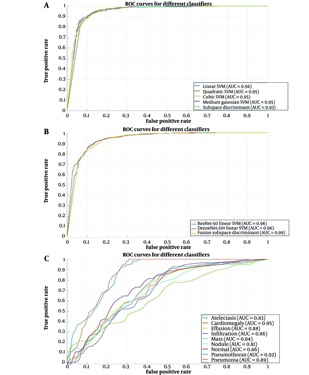
Figure 9A presents a graph comparing AUC values that illustrate the performance of the five classifiers applied to features derived from the fusion of the two models. These results underscore the proficiency of the fusion in extracting valuable features that improve the effectiveness of various machine learning classifiers. Figure 9B presents a graph that compares AUC-ROC values, illustrating the performance of the three best classifiers applied to features derived from ResNet-50, DenseNet-201, and the combination of both models. The LSVM classifiers from ResNet-50 and DenseNet-201 demonstrated strong performance, each with an AUC value of 0.96. Meanwhile, from the fusion of both models, ESD achieved the highest AUC-ROC value of 0.99. Figure 9C presents the ROC curve of eight lesions on the CXR dataset: Cardiomegaly, effusion, infiltrate, mass, nodule, atelectasis, pneumonia, and pneumothorax.
To comprehensively investigate the performance of our classifiers, we computed several key metrics across various experiments. To summarize the performance attributes, we identified the mean and SD of these metrics for different classifiers. Table 4 presents the mean ± SD values of each metric across all the evaluated classifiers in this study. The 95% confidence intervals (CI) indicate the statistical range in which the true metric value is expected to lie, based on 10-fold cross-validation results, providing a more robust understanding of model performance than a single average value. The relatively small SD across cross-validation folds (e.g., F1 score = 94.85 ± 0.56) further indicates stable and robust performance, reducing the likelihood of overfitting. Additionally, training and validation losses were monitored during model optimization. Both curves showed smooth convergence without divergence, suggesting proper generalization.
| Algorithms | Sensitivity rate (%) | Precision rate (%) | Specificity rate (%) | F1 score (%) | Computational time (s) |
|---|---|---|---|---|---|
| M-ResNet50 | 92.59 ± 0.32 | 89.91 ± 0.42 | 89.39 ± 0.35 | 90.93 ± 0.24 | 66.09 ± 70.83 |
| M-DenseNet201 | 91.58 ± 0.63 | 88.54 ± 0.74 | 88.79 ± 0.79 | 90.04 ± 0.53 | 40.04 ± 37.53 |
| Hybrid MR50 + MD201 | 95.95 ± 1.09 | 93.91 ± 0.37 | 93.91 ± 0.34 | 94.85± 0.56 | 26.98 ± 7.25 |
| [95.27, 96.63] | [93.68, 94.14] | [93.70, 94.12] | [94.50, 95.20] | [22.49, 31.47] |
Abbreviations: M-ResNet50, modified ResNet-50; M-DenseNet201, modified DenseNet-201.
a Values are expressed as mean ± standard deviation (SD) or 95% confidence intervals.
Table 5 represents the individual comparison of the computational speed across all the classifiers with the relevant models. Computational speed plays a crucial role in deep learning-based medical image analysis. The table emphasizes the computational times of the different models, demonstrating their efficiency in handling image classification. Some models exhibit higher accuracy but require longer processing times. Our proposed hybrid method balances computational efficiency and classification performance, ensuring optimal results.
| Classifiers | Computational Speed (s) | ||
|---|---|---|---|
| M-ResNet50 | M-DenseNet201 | Hybrid proposed model | |
| LSVM | 30.599 | 107.09 | 31.825 |
| QSVM | 32.112 | 22.671 | 35.337 |
| CSVM | 36.864 | 24.536 | 24.291 |
| MGSVM | 38.216 | 25.401 | 26.924 |
| ESD | 192.68 | 20.489 | 16.511 |
Abbreviations: M-ResNet50, modified ResNet-50; M-DenseNet201, modified DenseNet-201; LSVM, linear support vector machine; QSVM, quadratic support vector machine; CSVM, cubic support vector machine; MGSVM, medium Gaussian support vector machine; ESD, ensemble subspace discriminant.
Table 6 shows a comparison of some previous and recent state-of-the-art models and their performance metrics. Wang et al. utilized a CXR image dataset to classify the images and achieved 93.40% accuracy, 93.30% sensitivity, and 95.76% specificity. Furthermore, Wang et al. (22) modified an inception TL model to establish an AI algorithm and used a binary dataset, achieving 89.50% accuracy. Subsequently, Song et al. (23) obtained 93.0% accuracy. Perumal et al. (24) proposed a deep learning model named Inception Nasnet that achieved 94.3% accuracy. Furthermore, another study applied a deep learning-based image analysis called cardio-XAttentionNet, performing binary classification and achieving 85% accuracy. Moreover, Benmalek et al. (25) used CXR images from ResNet-18, InceptionV3, and MobileNetV2 for the experimental process and achieved 87.70% accuracy. In our work, we proposed a hybrid-based approach consisting of the fusion of features from the modified DL model that achieved a state-of-the-art accuracy of 95.9%.
| Reference | Accuracy | Sensitivity rate | Specificity rate | Precision rate | F1 score |
|---|---|---|---|---|---|
| Wang et al. (11) | 89.50 | 87.0 | 88.0 | - | - |
| Benmalek et al. (25) | 87.70 | 92.30 | 88.80 | 93.40 | - |
| Song et al. (23) | 93.0 | 93.0 | 88.80 | 93.40 | - |
| Wang et al. (22) | 93.40 | 93.30 | 95.76 | - | - |
| Perumal et al. (24) | 94.3 | 94.0 | - | 94.0 | - |
| Innat et al. (9) | 85.0 | 85.0 | - | 87 | 86.0 |
| Our proposed hybrid approach | 95.9 | 97.70 | 94.16 | 93.94 | 95.78 |
a Values are expressed as percentage.
Table 7 compares eight lesions (cardiomegaly, effusion, infiltrate, mass, nodule, atelectasis, pneumonia, and pneumothorax) from previous state-of-the-art models. We achieved better AUC values than the previous results (26-31). The most recent results were those of Kufel et al. (32), who achieved an AUC of 0.817 for atelectasis, whereas we achieved 0.881. For cardiomegaly lesions, Kufel et al. (32) achieved an AUC of 0.911, whereas we achieved 0.947. Considering all results, we have average AUC scores, and a recent study achieved an AUC of 0.843, whereas we achieved 0.889.
| Pathology Label | Yao et al. (26) | Wang et al. (27) | Shen and Gao (28) | Guendel et al. (29) | Yan et al. (30) | Baltruschat et al. (31) | Kufel et al. (32) | Ours |
|---|---|---|---|---|---|---|---|---|
| Atelectasis | 0.733 | 0.700 | 0.766 | 0.767 | 0.792 | 0.763 | 0.817 | 0.831 |
| Cardiomegaly | 0.856 | 0.810 | 0.801 | 0.883 | 0.881 | 0.875 | 0.911 | 0.947 |
| Effusion | 0.806 | 0.759 | 0.797 | 0.828 | 0.842 | 0.822 | 0.879 | 0.880 |
| Infiltration | 0.673 | 0.661 | 0.751 | 0.709 | 0.710 | 0.694 | 0.716 | 0.863 |
| Mass | 0.777 | 0693 | 0.760 | 0.821 | 0.847 | 0.820 | 0.853 | 0.843 |
| Nodule | 0.724 | 0.669 | 0.741 | 0.758 | 0.811 | 0.747 | 0.771 | 0.810 |
| Pneumonia | 0.684 | 0.658 | 0.778 | 0.731 | 0.740 | 0.714 | 0.769 | 0.885 |
| Pneumothorax | 0.805 | 0.799 | 0.800 | 0.846 | 0.876 | 0.840 | 0.898 | 0.919 |
| Average | 0.7614 | 0.745 | 0.775 | 0.807 | 0.830 | 0.727 | 0.843 | 0.872 |
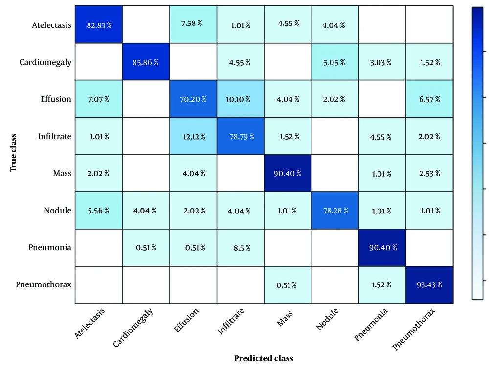
Figure 10 presents the confusion matrix for the eight lesions, showing the misclassification rates for each class separately. Overall, the model demonstrated high precision across most classes, with particularly strong performance for cardiomegaly (85.86%), pneumothorax (93.43%), and mass (90.4%). However, certain confusions were observed: Infiltrate was occasionally misclassified as cardiomegaly (12.12%) and pneumonia (2.02%), and effusion showed noticeable confusion with infiltrate (10.10%) and pneumothorax (6.57%), whereas nodule and atelectasis had minor misclassifications across multiple classes.
5. Discussion
In our study, we performed two types of experiments on two different datasets. The first dataset consists of only two classes: Normal and abnormal. The second dataset includes CXR images with eight lesions of abnormality, namely, cardiomegaly, effusion, infiltrate, mass, nodule, atelectasis, pneumonia, and pneumothorax. For diagnosis and classification, we developed a hybrid approach, which consists of more than one deep learning pretrained modified model. These models were trained using TL after separately applying the optimization technique, and several statistical analyses were used, including the Kruskal-Wallis test, ReliefF, ANOVA, chi-square test, and MRMR.
The deep learning models used in this study included ResNet-50 and DenseNet-201, which were trained using TL and achieved the best accuracy after these implementations. As presented in the experimental section above, we used various classifiers such as LSVM, QSVM, CSVM, MGSVM, and ESD models. The fusion of deep features and statistically selected handcrafted features was performed using feature-level horizontal concatenation. More explicitly, the deep features, extracted using fine-tuned deep learning models, were first optimized using the ACO algorithm, selecting a fixed number of relevant features. Meanwhile, the handcrafted features were selected by applying five statistical methods (MRMR, ANOVA, chi-square, Kruskal-Wallis, ReliefF). The union of the top-ranked features, based on repeated overlap, was extracted, resulting in a fixed-size statistical feature vector. Prior to fusion, both feature sets were converted to numerical matrix form and aligned row-wise per sample. The two feature matrices were then concatenated horizontally using MATLAB’s horzcat function to create a single composite feature vector.
While it is true that our approach builds upon existing models and selection techniques, which are based on ResNet-50, DenseNet-201, ACO, and statistical methods, the novelty of our work lies in the way we have strategically integrated these components into a unified and diagnostically meaningful framework, specifically optimized for CXR classification. We combine optimized deep features (via ACO) and statistically significant handcrafted features selected across five methods. To our knowledge, such a balanced and explainable hybrid fusion for CXR diagnosis has not been extensively explored. By fusing interpretable statistical features with deep features optimized through ACO, we improve both interpretability and classification accuracy, which is crucial in medical diagnostics. Last but not least, despite using multiple layers of processing, our method exhibits competitive or even reduced computational time compared to using single deep models alone, as demonstrated in Table 5.
For instance, the strength of our work is that we have achieved better results on both separate datasets and better accuracy than previous work on these datasets. We have also separately compared the achievements and used a proposed hybrid approach for both tasks. For the binary class of the CXR, we achieved the best accuracy at 95.9%, along with 97.70% sensitivity, 94.16% specificity, 93.94% precision, and 95.78% F1 score compared with other evaluation metrics. Our findings are higher after the comparison of eight abnormalities compared to the previous study, with an average AUC of 0.872 and higher for every individual class. Our hybrid model achieved 95.9% with a lower classification time of 16.511 seconds in ESD compared to baseline models. The proposed fusion pipeline can be generalized to other imaging domains where both interpretability and performance are essential.
The proposed method can be used for various other detection and classification tasks using magnetic resonance imaging and other types of datasets consisting of images. As previously mentioned, we have mapped different figures to provide a good representation of our results. First, we mapped the AUC curves of different classifiers in the first task and created a bar chart of the top 10 features selected based on the statistical analysis methods mentioned above. Second, we mapped the AUC curves of the eight lesions to better understand the outcomes of our hybrid approach on the CXR dataset (33, 34).
Unlike previous studies that solely depend on CNN feature extraction, our approach refines the feature set before classification, thereby improving both accuracy and interpretability. By fusing these optimized feature sets, our model effectively captures complex patterns in medical images, addressing challenges such as small lesion detection. Furthermore, traditional encoder–decoder networks involve high computational costs for up-sampling, but our method remains computationally efficient.
In conclusion, our research introduces a comprehensive approach for accurately classifying CXR images using the capabilities of deep learning models, specifically ResNet-50 and DenseNet-201, along with sophisticated feature selection techniques, which include the improved ACO algorithm and the five statistical analysis methods discussed in detail. The results were easier to interpret due to the thorough assessment of the importance of features provided by the systematic statistical analysis employing five different methodologies.
We have two primary classes in our dataset, normal and abnormal; however, for the abnormal class, we only have eight lesions to classify. Therefore, we also used the CXR dataset called CXR8 separately for mapping those lesions, namely, cardiomegaly, effusion, infiltrate, mass, nodule, atelectasis, pneumonia, and pneumothorax. Our proposed hybrid approach was trained on this type of dataset, which was a fine-tuned model for high sensitivity and specificity in detecting these conditions. Considering all aspects, this approach exhibits promise for improving medical imaging diagnostic capabilities by providing a reliable way to differentiate between normal and abnormal CXR images. This study has certain limitations despite the encouraging outcomes. The extent to which the conclusions can be applied broadly may be limited because the dataset used may not accurately represent the range of CXR images encountered in actual practice. To improve the model’s robustness and generalizability, future research is warranted to address these constraints by expanding the dataset to include a greater variety of CXR images from other sources. Moreover, realizing the full potential of deep learning models may require operating on larger datasets. Furthermore, the computational efficiency of the suggested method needs to be enhanced to make it more practicable for application in diverse clinical scenarios. In conclusion, its practical use would be greatly improved by incorporating the classification approach into multi-class classification for certain lung disorders, e.g., differentiating between different kinds of pneumonia or identifying other lung diseases such as COVID-19 and lung cancer. A comparison with an end-to-end fine-tuned CNN (e.g., CNN+FC+Softmax) will be explored as part of future work to further validate the advantage of our hybrid strategy.
