

1. Background
1.1. Diffusion Tensor Imaging (DTI)
1.2. Rotational Invariant Quantities


1.3. Segmentation Problems
1.4. Image Segmentation Methods
2. Objectives
3. Materials and Methods
3.1. Data Acquisition and Preprocessing
3.2. Parameters and Data Selection
3.3. CSF/Non-CSF Tissue Segmentation
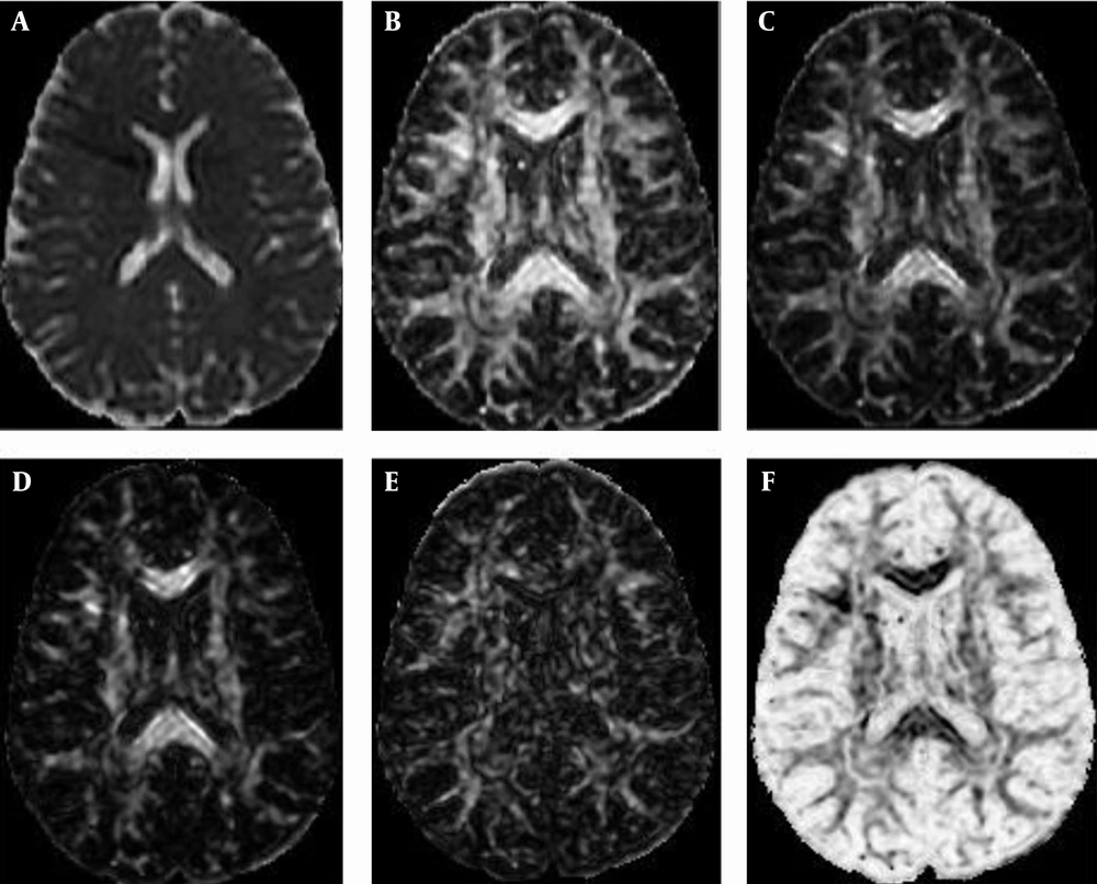
Some scalar indices of a human brain where A, Mean diffusivity; B, Fractional anisotropy; C, Rational anisotropy; D, Linear anisotropy; E, Planner anisotropy, and F, Spherical anisotropy.
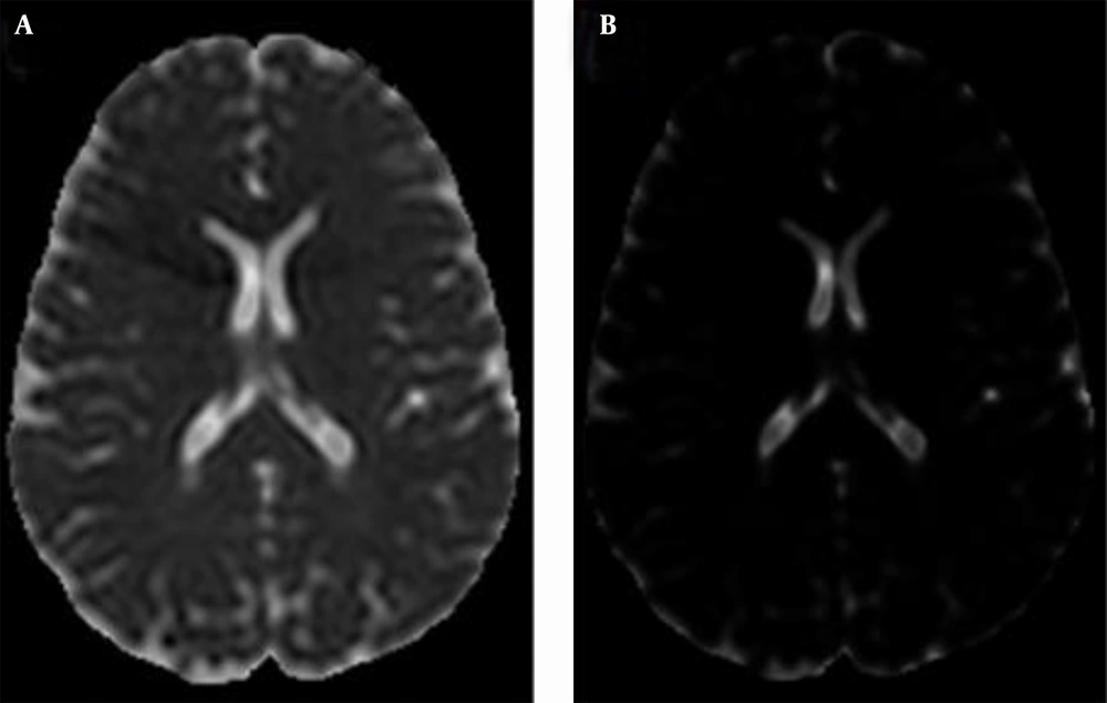
Cross-section in a human brain that shows A, The mean diffusivity image that is produced from the mean diffusivity scalar index; and B, The diffusion volume image that is produced from the diffusion volume scalar index for the same slice.
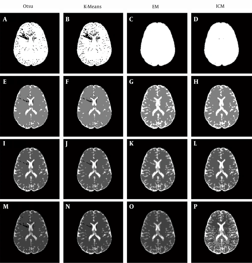
Clustering maps of an mean diffusivity image using different methods. A, Otsu2-MD; B, K-means2-MD; C, EM2-MD; D, ICM2-MD; E, Otsu3-MD; F, K-means3-MD; G, EM3-MD; H, ICM3-MD; I, Otsu4-MD; J, K-means4-MD; K, EM4-MD; L, ICM4-MD.
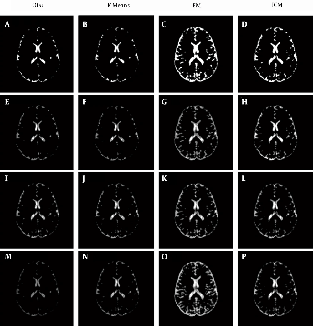
Clustering maps of a diffusion volume image using different methods. A, Otsu2-DV; B, K-means2-DV; C, EM2-DV; D, ICM2-DV; E, Otsu3-DV; F, K-means3-DV; G, EM3-DV; H, ICM3-DV; I, Otsu4-DV; J, K-means4-DV; K, EM4-DV; L, ICM4-DV.
3.4. WM/Non-WM Tissue Segmentation
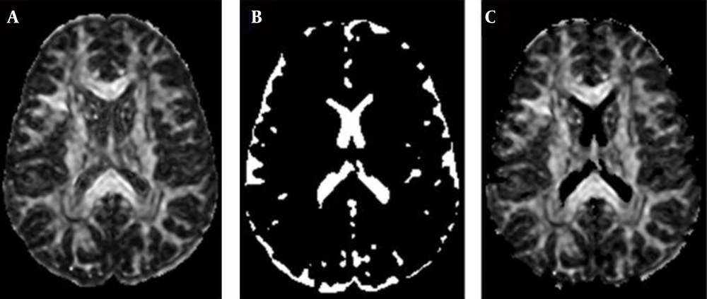
A, Normalized fractional anisotropy map; B, Cerebrospinal fluid clustering map (ICM2-DV clustering map); C, Normalized fractional anisotropy image after removing cerebrospinal fluid.
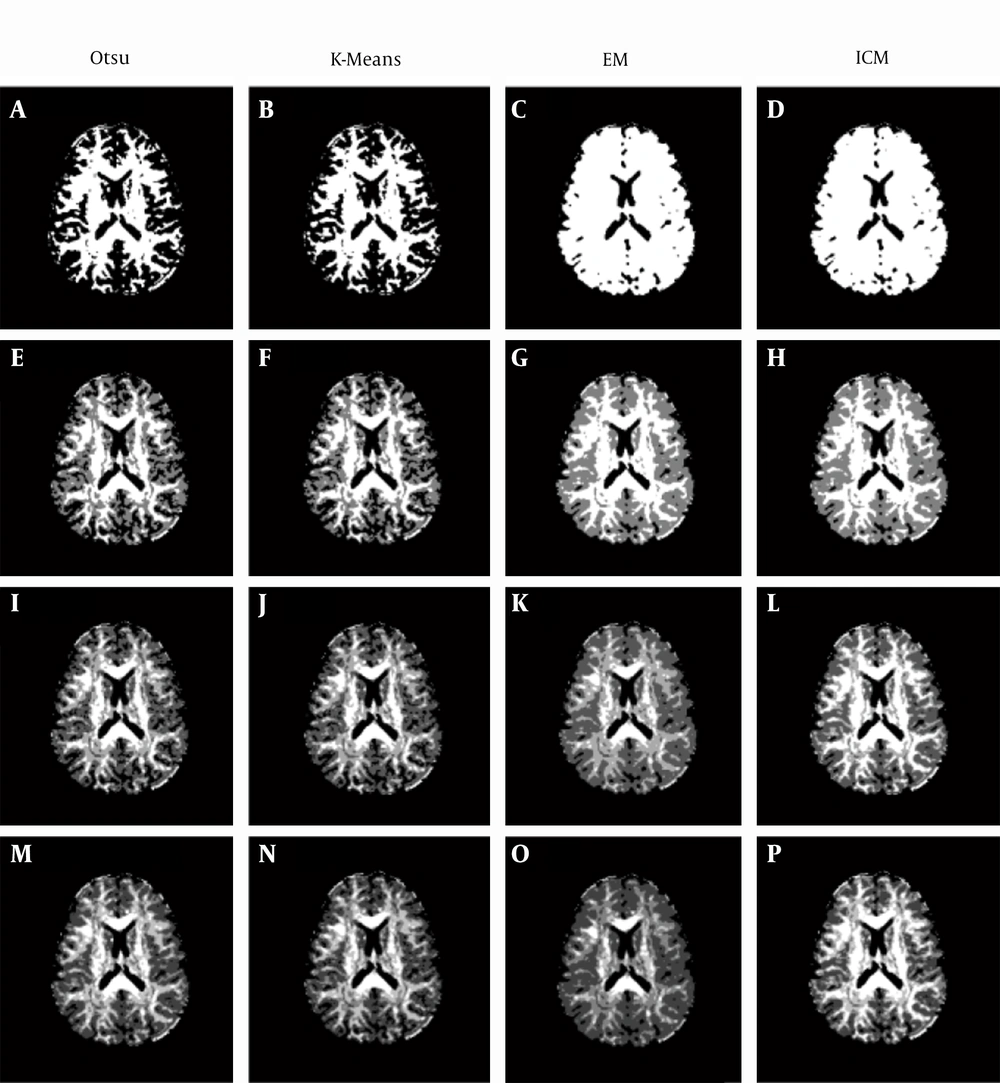
Clustering maps of an fractional anisotropy image using different methods. A, Otsu2-FA; B, K-Means2-FA; C, EM2-FA; D, ICM2-FA; E, Otsu3-FA; F, K-Means3-FA; G, EM3-FA; H, ICM3-FA; I, Otsu4-FA; J, K-Means4-FA; K, EM4-FA; L, ICM4-FA.
3.5. Brain Tissue Reconstruction
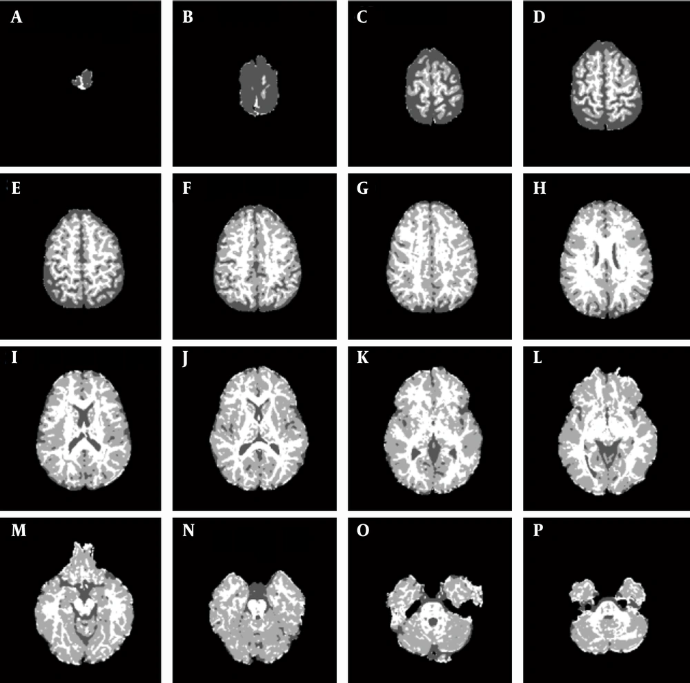
Clustering maps of the brain components at different levels with level ID in the corner (WM = White, GM = Light gray and CSF = Dark. A, level ID = 48; B, level ID = 45; C, level ID = 42; D, level ID = 39; E, level ID = 36; F, level ID = 33; G, level ID =30; H, level ID = 27; I, level ID = 24; J, level ID = 21; K, level ID = 18; K, level ID = 15; M, level ID = 12; N, level ID = 9; O, level ID = 6; P, level ID = 3.
4. Results
4.1. CSF/Non-CSF Tissue Segmentation Results
| # of Clusters | Otsu | K-Means | EM | ICM | ||||
|---|---|---|---|---|---|---|---|---|
| CSF (%) | RE (%) | CSF (%) | RE (%) | CSF (%) | RE (%) | CSF (%) | RE (%) | |
| 2 | 82.21 ± 24.28 | 391.61 ± 229.54 | 69.60 ± 29.83 | 327.84 ± 264.14 | 99.02 ± 0.06 | 472.50 ± 161.90 | 98.99 ± 0.06 | 472.34 ± 161.93 |
| 3 | 16.84 ± 3.27 | 7.79 ± 3.79 | 16.77 ± 3.23 | 8.13 ± 3.58 | 30.85 ± 3.80 | 76.25 ± 24.62 | 26.85 ± 2.81 | 54.49 ± 24.35 |
| 4 | 8.69 ± 4.00 | 52.48 ± 17.93 | 9.55 ± 2.75 | 48.95 ± 6.78 | 9.40 ± 5.44 | 46.19 ± 29.43 | 15.81 ± 3.24 | 48.35 ± 64.26 |
| 5 | 1.60 ± 3.01 | 91.34 ± 15.70 | 3.67 ± 2.22 | 79.92 ± 10.63 | 1.80 ± 0.49 | 89.76 ± 3.78 | 14.52 ± 3.68 | 66.75 ± 66.74 |
| 6 | 0.48 ± 0.78 | 97.28 ± 4.46 | 1.45 ± 0.32 | 91.99 ± 1.26 | 1.11 ± 0.11 | 93.72 ± 1.30 | 12.20 ± 2.34 | 41.28 ± 22.81 |
| 7 | 0.00 ± 0.00 | 100.00 ± 0.00 | 1.03 ± 0.12 | 94.24 ± 0.90 | 0.88 ± 0.08 | 95.04 ± 0.89 | - | - |
| 8 | 0.00 ± 0.01 | 99.99 ± 0.03 | 0.82 ± 0.11 | 95.39 ± 0.73 | 0.77 ± 0.10 | 95.69 ± 0.67 | - | - |
| 9 | 0.13 ± 0.28 | 99.29 ± 1.60 | 0.64 ± 0.13 | 96.44 ± 0.61 | 0.62 ± 0.08 | 96.52 ± 0.56 | - | - |
| 10 | 0.00 ± 0.00 | 100.00 ± 0.00 | 0.50 ± 0.06 | 97.20 ± 0.49 | 0.50 ± 0.08 | 97.23 ± 0.44 | - | - |
Abbreviations: CSF, cerebrospinal fluid; RE, relative error.
| # of Clusters | Otsu | K-Means | EM | ICM | ||||
|---|---|---|---|---|---|---|---|---|
| CSF (%) | RE (%) | CSF (%) | RE (%) | CSF (%) | RE (%) | CSF (%) | RE (%) | |
| 2 | 8.05 ± 2.92 | 57.78 ± 10.45 | 7.62 ± 2.85 | 60.10 ± 10.4 | 24.30 ± 3.50 | 38.98 ± 11.35 | 16.74 ± 3.53 | 8.86 ± 2.49 |
| 3 | 10.78 ± 3.08 | 42.29 ± 7.17 | 10.12 ± 2.92 | 45.90 ± 7.05 | 24.30 ± 3.50 | 38.98 ± 11.35 | 18.89 ± 3.12 | 10.63 ± 5.46 |
| 4 | 14.27 ± 3.20 | 22.01 ± 8.73 | 12.87 ± 2.82 | 30.06 ± 4.61 | 26.51 ± 3.07 | 57.02 ± 53.88 | 20.80 ± 3.25 | 20.03 ± 8.68 |
| 5 | 13.17 ± 3.22 | 27.79 ± 13.38 | 15.28 ± 3.27 | 16.82 ± 2.99 | 34.32 ± 4.62 | 99.65 ± 49.21 | 22.52 ± 3.13 | 29.58 ± 12.13 |
| 6 | 13.64 ± 4.53 | 28.23 ± 10.19 | 16.18 ± 3.49 | 11.86 ± 3.23 | 34.32 ± 4.62 | 99.65 ± 49.21 | 24.22 ± 3.02 | 39.28 ± 15.91 |
| 7 | 14.11 ± 2.40 | 22.67 ± 8.47 | 17.43 ± 2.79 | 8.64 ± 4.39 | 34.32 ± 4.62 | 99.65 ± 49.21 | - | - |
| 8 | 14.13 ± 2.55 | 22.37 ± 8.66 | 17.95 ± 2.89 | 8.02 ± 4.43 | 34.32 ± 4.62 | 99.65 ± 49.21 | - | - |
| 9 | 14.37 ± 3.76 | 22.08 ± 9.54 | 18.68 ± 3.13 | 9.63 ± 5.49 | 34.32 ± 4.62 | 99.65 ± 49.21 | - | - |
| 10 | 15.67 ± 2.60 | 14.39 ± 3.70 | 19.15 ± 3.20 | 11.49 ± 4.90 | 35.34 ± 4.11 | 104.24 ± 43.97 | - | - |
Abbreviations: CSF, cerebrospinal fluid; RE, relative error.
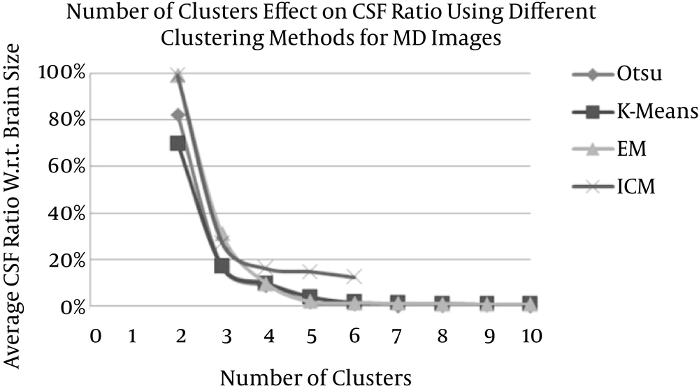
Average CSF ratio (with respect to total brain volume) versus various numbers of clusters for Otsu’s, K-means, EM, and ICM methods when employed for the MD map. (CSF, cerebrospinal fluid; MD, mean diffusivity).
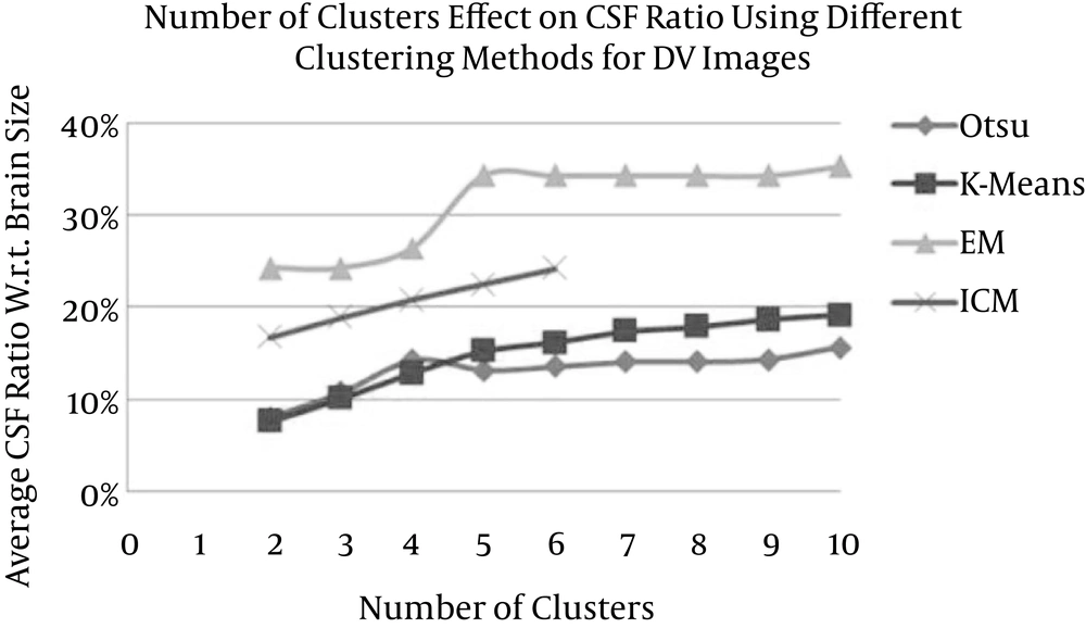
Average CSF ratio (with respect to total brain volume) versus various numbers of clusters for Otsu’s, K-means, EM, and ICM methods when employed for the DV map. (CSF, cerebrospinal fluid; DV, Diffusion Volume).
4.2. WM / Non-WM Tissue Segmentation Results
| # of Clusters | Otsu | K-Means | EM | ICM | ||||
|---|---|---|---|---|---|---|---|---|
| WM (%) | RE (%) | WM (%) | RE (%) | WM (%) | RE (%) | WM (%) | RE (%) | |
| 2 | 50.04 ± 3.12 | 44.81 ± 5.09 | 49.73 ± 3.18 | 43.98 ± 4.47 | 82.29 ± 3.53 | 129.95 ± 18.79 | 82.22 ± 3.52 | 131.47 ± 18.99 |
| 3 | 23.32 ± 1.22 | 38.95 ± 2.76 | 23.12 ± 1.38 | 39.53 ± 2.62 | 35.1 6± 0.69 | 11.60 ± 2.34 | 35.05 ± 1.13 | 4.77 ± 3.15 |
| 4 | 12.03 ± 0.96 | 68.52 ± 2.34 | 11.32 ± 0.71 | 70.36 ± 1.99 | 6.96 ± 0.42 | 81.70 ± 2.15 | 21.87 ± 0.89 | 38.94 ± 4.14 |
| 5 | 7.07 ± 0.60 | 81.46 ± 1.72 | 6.39 ± 0.43 | 83.27 ± 1.23 | 3.20 ± 0.28 | 91.58 ± 1.24 | 16.20 ± 1.05 | 54.75 ± 4.18 |
| 6 | 4.32 ± 1.60 | 88.63 ± 4.10 | 4.00 ± 0.27 | 89.55 ± 0.42 | 1.77 ± 0.27 | 95.32 ± 1.00 | 14.83 ± 0.86 | 58.55 ± 4.12 |
Abbreviations: WM, white matter; RE, relative error.
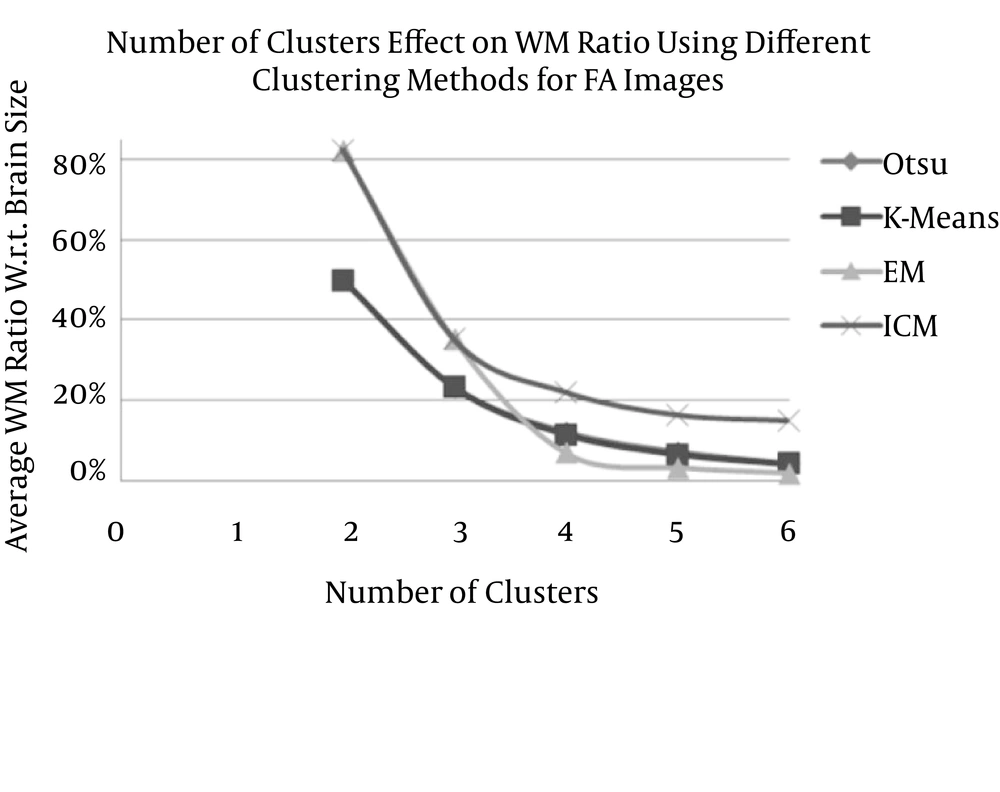
Average WM ratio (with respect to total brain volume) versus the number of clusters for Otsu’s, K-means, EM, and ICM methods when FA images are employed after removing CSF tissues. (CSF, cerebrospinal fluid; WM, white matter, FA, fractional anisotropy).

